Plate junctions: wave approach and experimental SEA

When a bending wave travelling on a wall or floor reaches a rigid junction with another plate, part of its energy is reflected and part is transmitted into the connected plates. The wave approach of Cremer et al. (1973), tabulated by Craik (1981, 1996) and collected in Hopkins (2007, Section 5.2.1.3), gives the transmission coefficient in closed form for the four most common junctions of thin, homogeneous, isotropic plates: the X, T, L and in-line junctions. Modelling the junction as a simply supported (pinned) massless beam forces an incident bending wave to generate only reflected and transmitted bending waves, with no conversion to in-plane waves, and the resulting coefficients are independent of frequency. That is what makes them convenient closed-form inputs for statistical energy analysis (SEA) and for the EN 12354 flanking-transmission model, where they feed the coupling loss factor ${\eta }_{ij}$ and the vibration reduction index $K_{ij}$.

That convenience has a price, and it is worth knowing before the number is used as though it were measured. A real junction’s $K_{ij}$ is frequency dependent, which is why ISO 10848 reports it per band and why EN 12354-1 Annex E tabulates band-dependent values. The wave approach needs plates thin relative to the bending wavelength, and enough modes in the band for the diffuse-field angular average of section 3 to mean anything, so it degrades at low frequency and on small elements. The in-plane conversion it discards grows with frequency and with junction complexity, so the closed form flatters heavy, stiff, complicated joints — the clip in section 2 shows exactly the precursor being neglected. And a massless pinned beam is a poor model of a junction that in reality carries mass and rotational stiffness. Section 5 hands one frequency-independent number straight to the EN 12354 model in place of a band-dependent one; when that matters, the measured counterpart is the Laboratory Flanking Transmission guide.

The object itself first: a T-junction where a 140 mm concrete floor runs into a continuous 200 mm wall. A junction_transmission result retains its plates, so res.plot_geometry() draws the junction to scale with the incident bending wave marked.

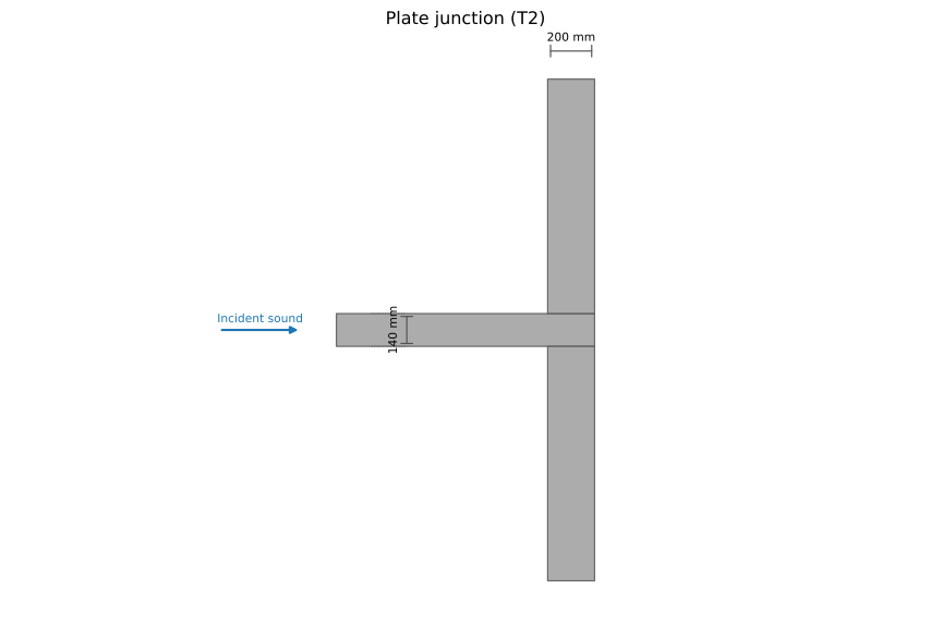
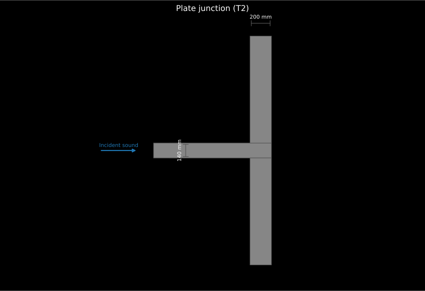
Drawn to scale: the incident bending wave arrives along the 140 mm floor, and everything the closed-form coefficients describe happens where it meets the continuous 200 mm wall.

Show the code for this figure

import matplotlib.pyplot as plt
from phonometry import junction_transmission

# A 140 mm concrete floor meeting a 200 mm wall at a T-junction.
res = junction_transmission("T2", 0.14, 3500.0, 320.0, 0.2, 3500.0, 460.0)
res.plot_geometry()
plt.show()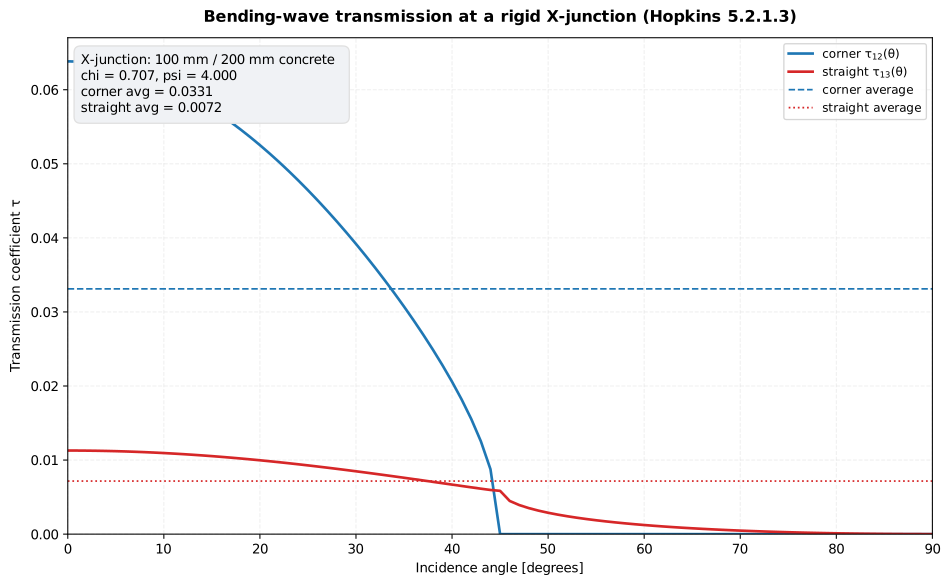

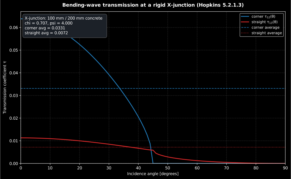
The sharpest feature of this figure is the cut-off. Beyond ${\theta }_{\text{co}}=\arcsin \chi =45°$ the heavier receiving plate has no propagating bending wave for the corner path to feed, so ${\tau }_{12}$ is exactly zero and stays there, while the straight path carries on to grazing incidence. That is why $\chi$ — a wavenumber ratio — and not $\psi$ sets the shape of the curve.

Show the code for this figure

import matplotlib.pyplot as plt
from phonometry import junction_transmission

# X-junction between a 100 mm and a 200 mm concrete plate (cL = 3200 m/s).
res = junction_transmission("X", 0.1, 3200.0, 240.0, 0.2, 3200.0, 480.0)
res.plot()  # tau(theta) for the corner and straight paths, with averages
plt.show()

1. Wave parameters chi and psi

With plate $i$ of thickness $h_i$, quasi-longitudinal wave speed $c_{L,i}$ and surface density ${\rho }_{s,i}$, the whole family of coefficients depends on just two dimensionless ratios (Cremer et al. 1973):

$$\chi =\frac{k_{B2}}{k_{B1}}={\left(\frac{{\rho }_{s2}{B}_1}{{\rho }_{s1}{B}_2}\right)}^{1/4}=\sqrt{\frac{h_1{c}_{L1}}{h_2{c}_{L2}}}=\sqrt{\frac{f_{c2}}{f_{c1}}}$$ $$\psi =\frac{B_2{k}_{B2}^2}{B_1{k}_{B1}^2}=\frac{h_2{c}_{L2}{\rho }_{s2}}{h_1{c}_{L1}{\rho }_{s1}}=\frac{{\rho }_{s2}{f}_{c1}}{{\rho }_{s1}{f}_{c2}}$$

$\chi$ is the ratio of the plates’ bending wavenumbers (equivalently the square root of their critical-frequency ratio) and sets the total-internal-reflection cut-off angle ${\theta }_{\text{co}}=\arcsin \chi$; $\psi$ is the ratio of their bending-moment mobilities. For identical plates both are 1.

from phonometry import junction_wave_parameters

chi, psi = junction_wave_parameters(0.1, 3200.0, 240.0, 0.2, 3200.0, 480.0)
#  -> (sqrt(0.5), 4.0)

2. Corner and straight-section coefficients

For an incident wave on plate 1, transmission around the corner (into the perpendicular plate 2) is ${\tau }_{12}(\theta )$ (Eq. 5.12), and transmission across the straight section (into the collinear plate 3, X- and T-junction (1) only) is ${\tau }_{13}(\theta )$ (Eq. 5.13). The corner coefficient is zero beyond the cut-off, ${\tau }_{12}(\theta )=0$ for $\chi <\sin \theta$. The junction constants $J_1$, $J_2$, $J_3$ select the geometry:

A T-junction has three plates, and which of them carries the incident wave is the whole distinction between its two cases. In T-junction (1) the wave arrives on one of the two collinear members, so it can go straight on into the collinear plate and round the corner into the branch. In T-junction (2) it arrives on the branch — the stem of the T — so both available paths are corners and there is no straight section at all. The opening figure of this page is a T2 for exactly that reason: the 140 mm floor is the branch, and the 200 mm wall runs through.

Junction	API string	$J_1$	$J_2$	$J_3$
X	"X"	1	1	1
T-junction (1)	"T1"	2	0.5	0.5
T-junction (2)	"T2"	2	2	—
L	"L"	4	1	—
in-line	—	*	*	*

* The in-line junction has no $J$ constants: it is a change of section, not a corner, so the geometry is one-dimensional. See below.

The straight section is undefined for the T-junction (2) and the L-junction.

Two plates parametrise all of this because the closed forms describe a symmetric junction, in which opposite plates are identical: for the X, plate 3 is a copy of plate 1 and plate 4 a copy of plate 2; for T-junction (1), plate 3 is a copy of plate 1; for T-junction (2), plate 4 is a copy of plate 2. The page’s own X-junction example is therefore a cross of two 100 mm plates and two 200 mm plates, not four different ones. That is a real restriction on a real building: a floor that differs above and below a junction, or a wall that continues in a different thickness, has no closed form here. Bound it with the two symmetric cases, or go to the EN 12354-1 Annex E empirical $K_{ij}$, or measure it. The L-junction needs no such caveat because it genuinely has two plates — and so, for a different reason, does the in-line junction.

The in-line junction: a change of section

The in-line junction is the one case on this page where the two plates are collinear, so there is no corner and the $J_1/J_2/J_3$ apparatus does not apply. A 100 mm slab continuing as a 200 mm slab is a common building situation, and it has its own closed form at normal incidence (Hopkins Eq. 5.14, after Cremer et al. 1973):

$${\tau }_{12}(0°)={\left[\frac{2(1+\chi )(1+\psi )\sqrt{\chi \psi }}{\chi (1+\psi {)}^2+2\psi (1+{\chi }^2)}\right]}^2$$

Only normal incidence is defined for it, for the geometric reason above; the module notes that the value is within 1 dB of the angular average whenever $\chi \ge 1$.

inline_transmission_coefficient(chi, psi) evaluates it. For the same 100 mm / 200 mm concrete pair as the figure above — $\chi =0.707$, $\psi =4.0$ from junction_wave_parameters — it returns 0.936, against exactly 1 for identical plates. Doubling the thickness of a continuing slab still passes 94 % of the incident power. That is the quantitative form of “a continuous plate transmits fully”, and it is why a change of section is a poor place to look for isolation.

import numpy as np
from phonometry import (
    corner_transmission_coefficient,
    straight_transmission_coefficient,
)

theta = np.radians(np.linspace(0.0, 90.0, 91))
tau12 = corner_transmission_coefficient(theta, chi, psi, "X")
tau13 = straight_transmission_coefficient(theta, chi, psi, "X")

The clip below runs this experiment in the time domain with the library’s 2D elastic FDTD solver: a bending packet on a 10 mm steel plate reaches an L-junction with an identical plate, and the corner splits it into the reflected and transmitted waves this section prices at ${\tau }_{12}(0°)=0.5$. The fast in-plane precursor racing down the receiving plate is the mode conversion the pinned-junction model deliberately leaves out.

A 4 kHz tone-burst force launches a bending-wave packet along a 10 mm steel plate. On the straight control plate the packet just runs on and nothing returns. At an L-junction with an identical perpendicular plate it splits: part reflects, part turns the corner as a bending wave descending the vertical plate, and a faster in-plane precursor races ahead, with the closed-form transmission coefficient of 0.50 at normal incidence and the diffuse vibration reduction index of 5.2 dB annotated.

Download the animation (WebM)

A 4 kHz tone-burst force launches a bending-wave packet along a 10 mm steel plate. On the straight control plate the packet just runs on and nothing returns. At an L-junction with an identical perpendicular plate it splits: part reflects, part turns the corner as a bending wave descending the vertical plate, and a faster in-plane precursor races ahead, with the closed-form transmission coefficient of 0.50 at normal incidence and the diffuse vibration reduction index of 5.2 dB annotated.

Download the animation (WebM)

3. Diffuse-field angular average

In a diffuse vibration field every angle of incidence is equally probable and the incident intensity carries a $\cos \theta$ obliquity factor, so the average transmission coefficient is ${\bar{\tau }}_{ij}={\int }_0^{\pi /2}{\tau }_{ij}(\theta )\cos \theta \mathrm{d}\theta$ (Eq. 5.6). For identical plates the algebra collapses to exact fractions that serve as the library’s first-principles oracle:

• X-junction corner and straight: ${\tau }_{ij}(\theta )={\cos }^2\theta /8$, so ${\bar{\tau }}_{ij}=1/12$;
• L-junction corner: ${\tau }_{ij}(\theta )={\cos }^2\theta /2$, so ${\bar{\tau }}_{ij}=1/3$;
• in-line junction: ${\tau }_{12}(0°)=1$ (a continuous plate transmits fully; for a change of section, inline_transmission_coefficient of section 2 applies).

from phonometry import angular_average_transmission_coefficient

angular_average_transmission_coefficient(1.0, 1.0, "X", section="corner")  # 1/12
angular_average_transmission_coefficient(1.0, 1.0, "L", section="corner")  # 1/3

The two directions obey the SEA consistency relationship (Eq. 5.7), ${\bar{\tau }}_{12}=\chi {\bar{\tau }}_{21}$, so only one direction needs to be computed.

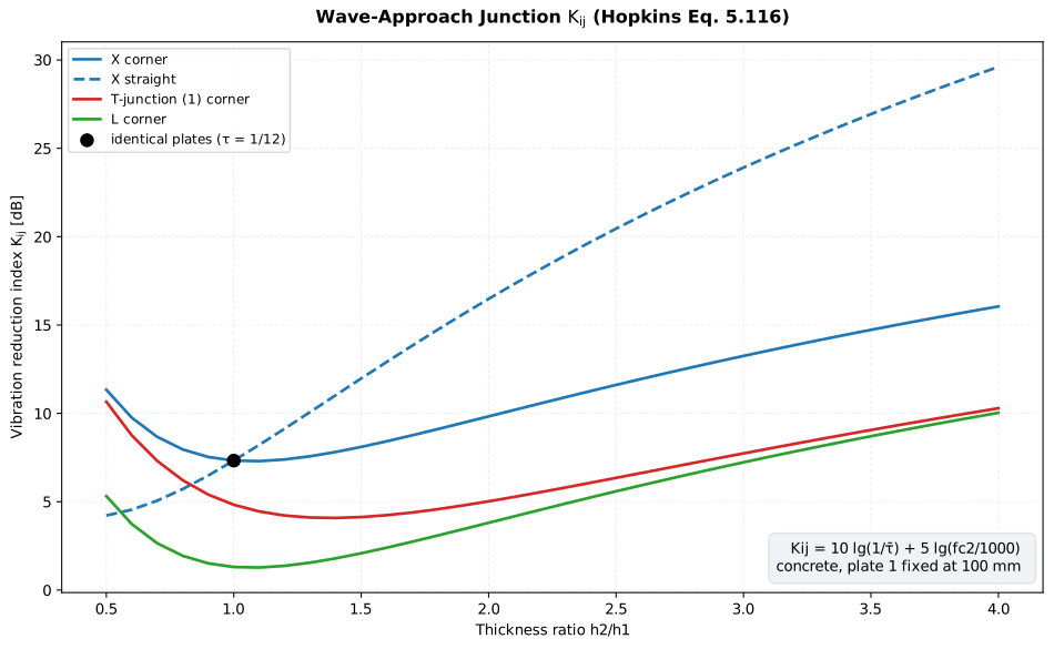
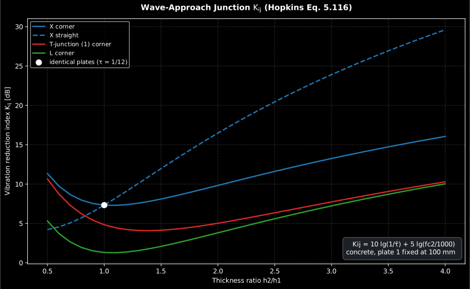
4. Coupling loss factor and vibration reduction index

The angular average is the bridge to the two junction descriptors used in SEA-based building models: the coupling loss factor (Eq. 2.154) ${\eta }_{ij}=c_{g,i}{L}_{ij}{\tau }_{ij}/(2{\pi }^{2}f{S}_i)$ and the wave-approach vibration reduction index (Eq. 5.116) $K_{ij}=10{\log }_{10}(1/{\tau }_{ij})+5{\log }_{10}(f_{c,j}/f_{\text{ref}})$ with $f_{\text{ref}}=1000\text{Hz}$ and $f_{c,j}$ the critical frequency of the receiving plate. Combined with the Eq. 5.7 reciprocity this form is symmetric, $K_{ij}=K_{ji}$, as EN 12354 requires of the junction descriptor. For the identical 100 mm concrete X-junction ($f_c\approx 203\text{Hz}$), $K_{ij}=10{\log }_{10}12+5{\log }_{10}(203/1000)\approx 7.3\text{dB}$.

from phonometry import (coupling_loss_factor, junction_transmission,
                        wave_vibration_reduction_index)

eta = coupling_loss_factor(1.0 / 12.0, group_velocity=200.0,
                           junction_length=4.0, frequency=500.0, plate_area=10.0)
res = junction_transmission("X", 0.1, 3200.0, 240.0, 0.1, 3200.0, 240.0)
kij = wave_vibration_reduction_index(res.corner_average,
                                     res.critical_frequency2)  # 7.33 dB
kij = res.corner_reduction_index  # the same, precomputed on the result

res.plot()   # tau(theta) for this junction's corner and straight paths (needs matplotlib)

$K_{ij}$ is also what ISO 10848 measures on a built junction: excite one element, read the velocity level difference on both, and normalize by the junction length, so the closed-form value above has a direct experimental counterpart.

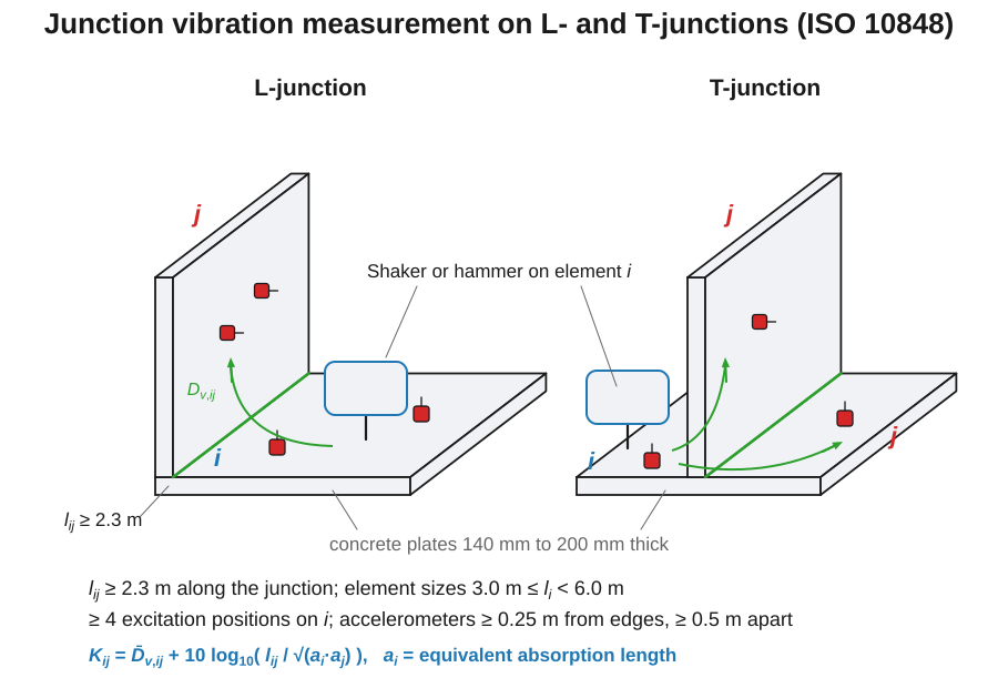
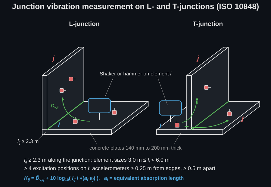
The junction descriptor is a design quantity: sweeping the receiving plate’s thickness shows how much a mass change at the junction buys. The corner paths stiffen quickly with a heavier receiving plate, while the straight (in-line) path of the X-junction rises fastest of all, since the perpendicular plates increasingly pin the junction line:

Show the code for this figure

import matplotlib.pyplot as plt
import numpy as np
from phonometry import junction_transmission, wave_vibration_reduction_index

# Concrete plates (cL = 3200 m/s, rho = 2400 kg/m3): plate 1 fixed at
# 100 mm, plate 2 swept from 50 mm to 400 mm.
h1, cl, rho = 0.1, 3200.0, 2400.0
ratios = np.linspace(0.5, 4.0, 36)
curves = {"X corner": [], "X straight": [], "T-junction (1) corner": [],
          "L corner": []}
for ratio in ratios:
    h2 = h1 * float(ratio)
    res_x = junction_transmission("X", h1, cl, rho * h1, h2, cl, rho * h2)
    curves["X corner"].append(res_x.corner_reduction_index)
    # Only the corner index is precomputed on the result; the straight path
    # is the angular average tau13 converted the same way.
    curves["X straight"].append(float(wave_vibration_reduction_index(
        res_x.straight_average, res_x.critical_frequency2)))
    res_t = junction_transmission("T1", h1, cl, rho * h1, h2, cl, rho * h2)
    curves["T-junction (1) corner"].append(res_t.corner_reduction_index)
    res_l = junction_transmission("L", h1, cl, rho * h1, h2, cl, rho * h2)
    curves["L corner"].append(res_l.corner_reduction_index)

fig, ax = plt.subplots()
for label, values in curves.items():
    ax.plot(ratios, values, "--" if label == "X straight" else "-", label=label)
# The identical-plate X-junction: Kij = 10 lg 12 + 5 lg(fc2/1000).
res_eq = junction_transmission("X", h1, cl, rho * h1, h1, cl, rho * h1)
ax.scatter([1.0], [res_eq.corner_reduction_index], zorder=6,
           label="identical plates (tau = 1/12)")
ax.set_xlabel("Thickness ratio h2/h1")
ax.set_ylabel("Vibration reduction index Kij [dB]")
ax.set_title("Wave-approach junction Kij (Hopkins Eq. 5.116)")
ax.legend()
plt.show()

5. Worked example: feeding Kij into EN 12354

The number this page predicts is exactly what the EN 12354-1 flanking model consumes. Take the 100 mm / 200 mm concrete X-junction of section 2’s $\tau (\theta )$ figure: its corner path gives $K_{12}=9.8\text{dB}$. Handing it to flanking_element in place of a tabulated Annex E value prices the junction’s three flanking paths and their effect on the apparent rating:

from phonometry import building, junction_transmission

# The 100 mm / 200 mm concrete X-junction of the tau(theta) figure:
res = junction_transmission("X", 0.1, 3200.0, 240.0, 0.2, 3200.0, 480.0)
k12 = res.corner_reduction_index                     # 9.8 dB (corner path)

# Feed it to the EN 12354-1 simplified model as this junction's Kij:
ff, df, fd = building.flanking_element(
    label="floor", r_flanking=49.0, r_separating=57.0,
    k_ff=k12, k_fd=k12, k_df=k12, separating_area=11.5, coupling_length=4.5)
pred = building.predicted_airborne_insulation(r_direct=57.0,
                                              flanking_paths=[ff, df, fd])
print(round(pred.r_prime_w, 1))                      # 55.4  (Rw 57 direct)
print(pred.dominant.label, round(pred.dominant.fraction, 2))   # Dd 0.68

One junction with a moderate $K_{ij}$ already trims 1.6 dB off the direct $R_w=57\text{dB}$; a full building repeats this for every junction, which is the EN 12354 prediction guide.

The measured, EN 12354 counterpart of $K_{ij}$ (from the direction-averaged velocity level difference) is the separate flanking-transmission vibration_reduction_index; this page is the closed-form predicted value from the wave approach.

6. Experimental SEA: coupling loss factors from measured energies

Everything above is the predictive route: a coupling loss factor derived from a wave model of the junction. Real joints — welds, bolt rows, spot welds, adhesives — are not tractable that way, and the experimental route inverts the steady-state SEA power balance from measured subsystem energies instead (Norton & Karczub 2003, Sections 6.3.3 and 6.3.4). For two subsystems,

$${\Pi }_1=\omega \left[({\eta }_1+{\eta }_{12})E_1-{\eta }_{21}{E}_2\right](6.10)$$ $$0=\omega \left[({\eta }_2+{\eta }_{21})E_2-{\eta }_{12}{E}_1\right](6.11)$$

with $E_i=M_i⟨v_i^2⟩$ the band energy of subsystem $i$ (its mass times the space- and time-averaged mean-square velocity). Drive subsystem 1 only, add the SEA consistency (reciprocity) relationship $n_1{\eta }_{12}=n_2{\eta }_{21}$ (Eq. 6.8), and both coupling loss factors follow from the two measured energies (Eq. 6.15):

$${\eta }_{12}=\frac{{\eta }_2{E}_2}{E_1-E_2{n}_1/n_2},{\eta }_{21}={\eta }_{12}\frac{n_1}{n_2},{\Pi }_{\text{in}}=\omega ({\eta }_1{E}_1+{\eta }_2{E}_2)$$

The input power collapses to the total dissipated power, as it must in the steady state: substituting Eq. (6.11) into Eq. (6.10) cancels the two coupling terms exactly, which is a free check on any measurement — and one to run on real data, not only on paper.

The measurement those symbols stand for

$E_i$ and ${\Pi }_{\text{in}}$ are measured quantities, and the inversion is only as good as they are. Norton’s section 6.6.4 describes the experiment; the requirements below are the ones that decide whether a result exists.

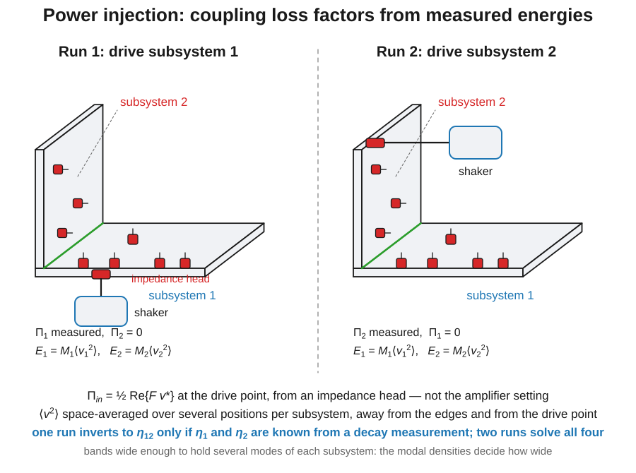
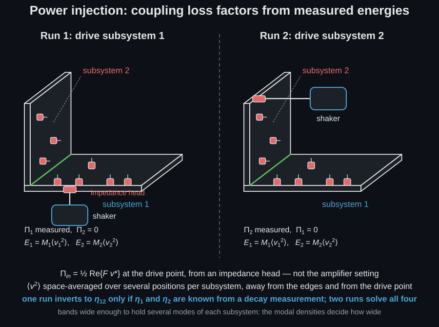
• Measure the injected power, do not infer it. Drive through a force transducer or an impedance head so that ${\Pi }_{\text{in}}=\frac{1}{2}\mathrm{Re}\{F{v}^{\ast }\}$ is formed at the drive point (Norton Eq. 6.50). Taken from the cross-spectrum of the force and velocity signals it is a time average and behaves well under broadband random excitation; taken from $\mathrm{Re}\{Z\}$ it does not, because the impedance is small exactly at a resonance and the loss factor estimate then inherits a large error.
• Space-average the velocities. $⟨v_i^2⟩$ is a space and time average, so it takes several accelerometer positions per subsystem, away from the edges and away from the drive point, and the excitation is repeated at several randomly chosen drive points so that the single-point excitation satisfies the statistical-independence assumption the model rests on.
• Choose bands that hold several modes. The SEA balance is an average over the modes in a band, so the band must contain enough of them — which is what the modal densities computed in this section are for, and why the same section computes them.
• Get ${\eta }_1$ and ${\eta }_2$ independently, or drive twice. The single-drive inversion of Eq. (6.15) takes the internal loss factors as inputs. They come from a separate experiment on the decoupled subsystems: a reverberation-decay measurement, or the steady-state energy-flow technique of Norton 6.5.3 ($\eta ={\Pi }_{\text{in}}/(\omega E)$, which needs the same input-power measurement again). If neither is available, drive each subsystem in turn instead — the two-drive scheme below, which needs no prior value at all.
• Keep the boundary losses out. The two-subsystem model assumes the energy flowing out of the pair at its far boundaries is negligible: fine wire point supports or foam pads approximating free-free conditions are what the literature uses. Mass loading, contact damping and exciter-structure feedback at the drive point are the same errors the mobility guide’s transducer section quantifies, and they apply here unchanged.
• Read the coupling against the damping. The figure’s own acceptance test: the coupling loss factors should sit at least an order of magnitude below the internal loss factors, or the subsystems are not weakly coupled and the model does not hold. PowerInjectionResult.coupling_strength reports that ratio.

power_injection_clf performs that inversion, with the modal densities of Norton Section 6.4.1 alongside it: flat_plate_modal_density (Eq. 6.25), bar_modal_density (6.23), beam_modal_density (6.24) and cylindrical_shell_modal_density (6.27 to 6.29, the Szechenyi approximations in three regimes about the ring_frequency of Eq. 6.26). The flat-plate expression $n(f)=S\sqrt{12}/(2c_{L}t)$ is the same quantity as EN 12354-4’s $n=\pi S{f}_c/c_0^2$ used by the flanking model, only parametrised by the plate itself rather than by its critical frequency.

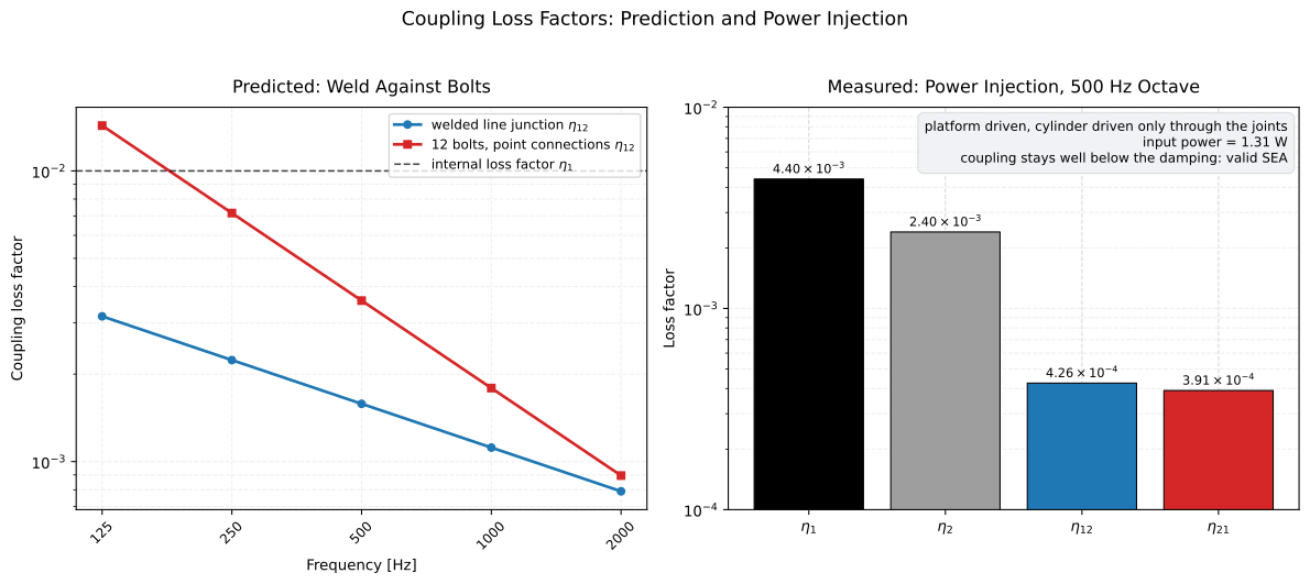
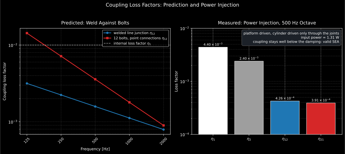
Left: two ways of joining the same two plates. Right: the loss-factor budget inverted from a pair of measured velocities; the coupling stays an order of magnitude below the damping, which is the condition for a two-subsystem SEA model to be trustworthy.

Show the code for this figure

import math
import matplotlib.pyplot as plt
import numpy as np
from phonometry import (
    coupling_loss_factor,
    cylindrical_shell_modal_density,
    flat_plate_modal_density,
    plate_bending_stiffness,
    point_connection_coupling_loss_factor,
    power_injection_clf,
    right_angle_transmission_coefficient,
)
from phonometry.vibration.structural.point_mobility import plate_bending_wave_speed

rho, nu, young = 2700.0, 0.33, 7.1e10                 # aluminium
cl = math.sqrt(young / (rho * (1.0 - nu**2)))         # 5432 m/s (Eq. 6.25)
bands = np.array([125.0, 250.0, 500.0, 1000.0, 2000.0])

# Predicted: a 3 mm x 2.5 m x 1.2 m plate meeting a 5.5 mm x 2.0 m x 1.2 m
# plate at right angles along the 1.2 m edge, welded and then bolted.
h1, h2, area1, length = 0.003, 0.0055, 2.5 * 1.2, 1.2
tau = right_angle_transmission_coefficient(h1, h2, density1=rho, density2=rho,
                                           wave_speed1=cl, wave_speed2=cl)
cb = plate_bending_wave_speed(bands, plate_bending_stiffness(young, h1, nu),
                              rho * h1)
welded = [float(coupling_loss_factor(tau, 2.0 * c, length, f, area1))
          for c, f in zip(cb, bands, strict=True)]
bolted = point_connection_coupling_loss_factor(
    bands, 12, thickness1=h1, thickness2=h2, surface_density1=rho * h1,
    surface_density2=rho * h2, wave_speed1=cl, wave_speed2=cl,
    plate_area1=area1)

# Measured: a 5 mm platform driven directly, a 3 mm cylinder driven only
# through the joints; 27.2 and 13.2 mm/s in the 500 Hz octave.
t_p, t_c, radius = 0.005, 0.003, 0.75
area_c = 2.0 * math.pi * radius * 2.0
area_p = 3.5 * 3.0 - math.pi * radius**2
sea = power_injection_clf(
    500.0, rho * t_p * area_p * 0.0272**2, rho * t_c * area_c * 0.0132**2,
    4.4e-3, 2.4e-3,
    flat_plate_modal_density(area_p, t_p, cl),
    float(cylindrical_shell_modal_density(500.0, area_c, t_c, radius, cl)[0]))

print(f"{float(sea.coupling_loss_factor12[0]):.2e}")   # 4.26e-04
print(f"{float(sea.coupling_loss_factor21[0]):.2e}")   # 3.91e-04
print(round(float(sea.input_power[0]), 2))             # 1.31 W
sea.plot()
plt.show()

Two closed forms sit between the two routes and are what a measured value is normally compared against. right_angle_transmission_coefficient gives the wave transmission coefficient of a right-angle plate junction without any angular integration (Eqs. 6.53 to 6.55, after Bies & Hamid and Cremer et al.); feeding it to coupling_loss_factor reproduces Norton Eq. (6.52) identically, because that equation and Hopkins Eq. (2.154) are the same expression once $c_g=2c_B$. And point_connection_coupling_loss_factor covers plates joined at $N$ discrete points instead of along a line (Eq. 6.56). Which one applies is decided by the bending wavelength: use the point form when it is shorter than the joint length, and the line form when it is longer. The two differ in slope as well as in level, $1/f$ against $1/\sqrt{f}$, so bolting and welding are not interchangeable across the spectrum.

When no independent value of the internal loss factors is available, the single-drive inversion is underdetermined, and the classical power-injection method drives each subsystem in turn while measuring both energies each time — the two states the rig diagram above draws. That gives four equations for ${\eta }_1$, ${\eta }_2$, ${\eta }_{12}$ and ${\eta }_{21}$ with no prior assumption at all, which power_injection_matrix solves band by band, taking the two energy pairs and the two injected powers and needing no modal density. It costs one extra run and it removes the measurement that is usually hardest to get (the decoupled decay), which is why it is the classical form. Run on the platform-and-cylinder example of the figure above it returns a modal_density_ratio of 0.919, against a geometric flat_plate_modal_density / cylindrical_shell_modal_density of 0.919 for the same structures — the two agreeing is the check.

Reciprocity then becomes a check on the measurement rather than an input: PowerInjectionResult.modal_density_ratio is a property, not a function, and it returns only the $n_1/n_2$ implied by the measured coupling loss factors, ${\eta }_{21}/{\eta }_{12}$. Making it a check is the reader’s step: compare it against the ratio built from the geometry with flat_plate_modal_density and its siblings, and a large disagreement means the subsystem boundaries were drawn in the wrong place. coupling_strength is the other diagnostic on the same result, and says whether the weak-coupling assumption the inversion rests on holds at all.

What this guide covers

• Covered

  The frequency-independent, rigid-junction transmission coefficients of Cremer, Heckl & Ungar (1973), tabulated by Craik (1981/1996) and collected in Hopkins (2007, Section 5.2.1.3), for the X, T, L and in-line junctions of thin, homogeneous, isotropic plates: the wave parameters $\chi$/$\psi$, the corner and straight-section coefficients ${\tau }_{12}(\theta )$/${\tau }_{13}(\theta )$, their diffuse-field angular average, the SEA coupling loss factor and the wave-approach vibration reduction index $K_{ij}$, via junction_wave_parameters, corner_transmission_coefficient, straight_transmission_coefficient, angular_average_transmission_coefficient, inline_transmission_coefficient, coupling_loss_factor, wave_vibration_reduction_index and junction_transmission.

  Section 6 covers the experimental route of Norton & Karczub Chapter 6: the two-subsystem power balance and its in-situ inversion (power_injection_clf, power_injection_matrix), the modal densities of bars, beams, flat plates and thin-walled cylindrical shells with the ring_frequency they are split about (bar_modal_density, beam_modal_density, flat_plate_modal_density, cylindrical_shell_modal_density), and the two closed forms that sit between the routes (right_angle_transmission_coefficient, point_connection_coupling_loss_factor).

• Not covered

  This predicted $K_{ij}$ is a closed-form idealisation for a rigid, simply supported junction, not a measurement: the measured, empirical $K_{ij}$ from a direction-averaged velocity level difference (ISO 10848) is the separate vibration_reduction_index of the Laboratory Flanking Transmission guide. The straight-section coefficient ${\tau }_{13}$ is undefined for the T-junction (2) and L-junction geometries, which have no collinear third plate, so only the corner path applies there. The tabulated coefficients also assume a symmetric junction (opposite plates identical), and there is no closed form here for one that is not. On the experimental side, the inversion of section 6 is written for two subsystems only, and PowerInjectionResult.modal_density_ratio is a consistency check the reader performs rather than one the library automates.

See also

• Predicting Sound Insulation (EN 12354): the flanking model that consumes $K_{ij}$ junction by junction.
• Laboratory Flanking Transmission (ISO 10848): the measurement of $K_{ij}$ from velocity level differences, the empirical counterpart of this page’s closed forms.
• Structure-borne sound power of equipment (EN 15657): the source power that these junction transmissions carry through a building.
• Mechanical mobility and the FRF family (ISO 7626-1): the plate mobilities behind the wave parameters.
• API reference: vibration.structural.junction_transmission.
• Theory: Point mobilities and radiation efficiency: the mobility picture behind a junction, and the radiation efficiency each element carries.

References

• Craik, R. J. M. (1996). Sound transmission through buildings using statistical energy analysis. Gower. The SEA treatment of building sound transmission with the tabulated bending-wave transmission coefficients for X, T, L and in-line junctions used here (Eqs 5.12/5.13). ISBN 978-0-566-07572-5.
• Cremer, L., Heckl, M., & Ungar, E. E. (1973). Structure-borne sound: Structural vibrations and sound radiation at audio frequencies (1st ed.). Springer. https://doi.org/10.1007/978-3-662-10118-6The original derivation of the wave parameters chi and psi (Eqs 5.10/5.11 in Hopkins) and the in-line normal-incidence transmission coefficient. ISBN 978-3-540-06002-4.
• Hopkins, C. (2007). Sound insulation. Butterworth-Heinemann. https://doi.org/10.4324/9780080550473Section 5.2.1.3 collects the rigid X, T, L and in-line junction coefficients, the angular average (Eq. 5.6), the SEA consistency relationship (Eq. 5.7), the coupling loss factor (Eq. 2.154) and the wave-approach Kij (Eq. 5.116) implemented on this page. ISBN 978-0-7506-6526-1.
• Norton, M. P., & Karczub, D. G. (2003). Fundamentals of noise and vibration analysis for engineers (2nd ed.). Cambridge University Press. https://doi.org/10.1017/CBO9781139163927Chapter 6 gives the two-subsystem SEA power balance (Eqs. 6.10, 6.11), the consistency relationship (Eq. 6.8), the in-situ inversion of the coupling loss factors from measured energies (Eq. 6.15), the modal densities of bars, beams, flat plates and thin-walled cylindrical shells (Eqs. 6.23-6.29) and the closed-form right-angle and point-connection coupling loss factors (Eqs. 6.52-6.56) implemented on this page. ISBN 978-0-521-49913-2.