Multiple-shock whole-body vibration (ISO 2631-5)

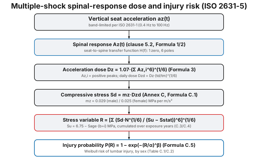
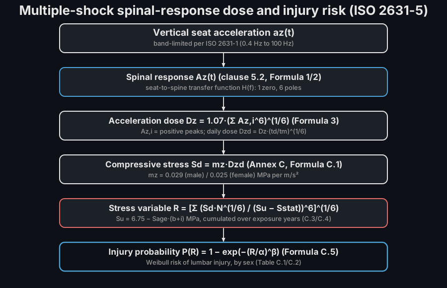
Vibration that contains repeated mechanical shocks (off-road vehicles, high-speed marine craft, earth-moving machinery) loads the lumbar spine far more than its equivalent r.m.s. level suggests. ISO 2631-5:2018 predicts the resulting spinal response and the risk of lumbar injury from the measured vertical seat acceleration. phonometry implements the normative Clause 5 spinal-response model and the Annex C health-effect assessment. (The Annex A / Annex E finite-element model is distributed by ISO as separate software and is out of scope here.)

The boundary with the basic method is explicit. ISO 2631-1 declares its r.m.s. evaluation normally sufficient up to a crest factor of 9, and offers the running r.m.s./MTVV and the VDV beyond it; ISO 2631-5 is the additional method for the regime past those, where the record contains repeated shocks. Its clause 4 then splits that regime in two: severe conditions with possible free fall or loss of contact with the seat and a dominant z-axis (military off-road vehicles, high-speed marine craft) use the clause 5 model implemented here, while less severe conditions in which the occupant stays seated throughout (tractors, forestry and earth-moving machinery on rough ground) belong to the Annex A finite-element model. In case of doubt the delineation is quantitative: when the band-limited vertical peak acceleration exceeds 9.81 m/s² (1 g, the free-fall threshold), clause 5 and Annex C apply.

1. Getting the record (clauses 5.1.2 and 5.1.4)

Everything below starts from a measured $a_z(t)$, and ISO 2631-5 adds four acquisition requirements on top of the ISO 2631-1 ones, each of them specific to shock exposure.

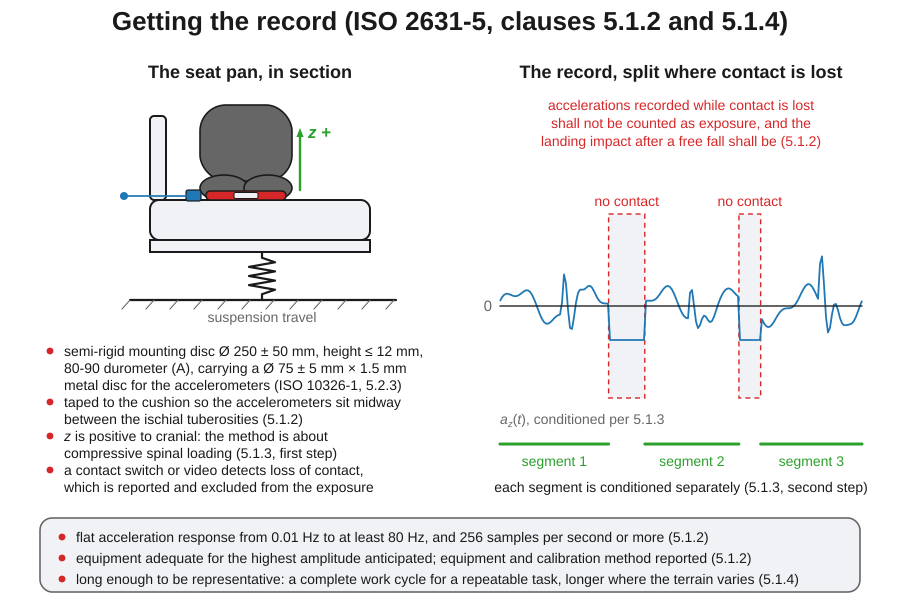
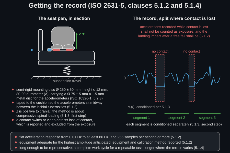
Where (5.1.2). $a_z(t)$ is measured at the interface between the seat and the ischial tuberosities. The measurement location on the seat and the design of the accelerometer disc on the seat pad follow ISO 10326-1: a semi-rigid moulded disc of 250 ± 50 mm diameter and at most 12 mm height, 80 to 90 durometer (A-scale), with a centre cavity holding a 75 ± 5 mm diameter, 1.5 mm thick metal disc that the accelerometers are attached to, taped to the cushion so that the transducers sit midway between the tuberosities (5.2.3 of that standard). The subject stays seated throughout data collection and does not rise from the seat.

Loss of contact (5.1.2). Contact switches, video recordings or another method detect loss of contact between the subject and the seat surface. Accelerations measured while contact is lost shall not be counted as exposure, and the loss of contact shall be detected and reported; the impact on landing after a free fall — the motion of the person and of the seat — shall be fully taken into account. This is the instrumentation that the severe regime of clause 4 above actually requires, and it is what makes an ISO 2631-5 record different from an ISO 2631-1 one.

The chain (5.1.2). The accelerometers and measuring equipment shall be appropriate for the highest amplitudes anticipated over the measurement period. The digitised record should have a flat acceleration response from 0.01 Hz to at least 80 Hz, and a sampling rate of 256 samples per second or greater can be necessary depending on the anti-aliasing method used — which is where the fs = 256.0 of the worked example below comes from. Details of the measurement equipment, including the calibration method used, shall be provided.

How long (5.1.4). The record shall be long enough for the measured multiple shocks to be typical of the exposure being assessed. Shock events may be infrequent, so the duration has to be estimated from how variable the impacts are: where a few severe shocks sit among many small ones, a longer record is needed to have a reasonable probability of capturing them. A complete work cycle is representative for a repeatable task such as a mine haul truck; for non-repeatable ones — off-road travel, military transport — the sufficient duration depends on the variability of the terrain. Trials that expose people to repeated shock need their own risk assessment, and shorter measurements first.

2. Conditioning the record (clause 5.1.3)

The conditioning is six ordered steps, and two of them contradict the advice a reader would otherwise give themselves.

1. Check the sign. The whole method is about compressive spinal loading, so the z axis must be positive to cranial: upward positive, in the basicentric system for seated persons. A sign error inverts which peaks are counted.
2. Cut out the parts with no contact between the accelerometer disc on the seat pad and the subject. This splits the record into separate parts, and the remaining steps are applied to each part separately.
3. Check the anti-aliasing if the data were resampled after acquisition. NOTE 1 warns that common data-processing packages apply suitable filters automatically, but that it is important to verify that they did.
4. Offset-correct so that the recorded acceleration reads (0 ± 0.1) m/s² with the accelerometer at rest. The clause then adds the warning: subtraction of the mean may not be appropriate if the recorded acceleration is asymmetric — and a shock record is asymmetric by construction, which is exactly the case a mean subtraction gets wrong.
5. Taper — a cosine taper over several seconds, for instance — if the accelerometer was in motion at the start or the end of the recording, before the band limiting.
6. Band-limit with a second-order Butterworth high pass at 0.01 Hz and a fourth-order Butterworth low pass at 80 Hz. The band-limiting and weighting filters of ISO 2631-1 shall not be applied.

The last step is where the number is won or lost. NOTE 2 gives the reason in numbers: free-fall periods above 0.5 s have been observed on fast naval craft, and a 0.5 Hz high pass drags the −1 g of the free fall back to zero before the impact arrives, so the impact peak is offset by up to +1 g and the calculated dose is wrong by of order 10 %. Abrupt changes in terrain contour can do the same. The 0.01 Hz corner exists to keep the free fall in the record.

import numpy as np
from scipy.signal import butter, filtfilt

# The clause 5.1.3 band limiting, on a record already offset-corrected and
# split at the loss-of-contact boundaries.
fs = 256.0
high = butter(2, 0.01, "high", fs=fs, output="sos")   # 2nd order, 0.01 Hz
low = butter(4, 80.0, "low", fs=fs, output="sos")     # 4th order, 80 Hz
print(high.shape, low.shape)                          # (1, 6) (2, 6)

3. Spinal response (clause 5.2)

A seat-to-spine transfer function $H(f)$ (one complex zero and six complex poles, unity transmissibility at 0 Hz and a resonance near 5 Hz) maps the conditioned seat acceleration to the vertical spinal response $A_z(t)$ (Formula 1/2):

$$A_z(t)={\mathcal{F}}^{-1}\left[H(f)\mathcal{F}[a_z(t)]\right].$$

The conditioning of section 2 is not optional here: because $H$ is unity at 0 Hz by design, a DC offset — the 1 g gravity component of a DC-coupled accelerometer, say — passes straight into $A_z(t)$ and corrupts the positive response peaks the dose is built from.

from phonometry import vibration

# The transmissibility peaks near the ~5 Hz spinal resonance.
print(round(abs(vibration.seat_to_spine_transfer([2.0])[0]), 2))  # 1.06
print(round(abs(vibration.seat_to_spine_transfer([5.0])[0]), 2))  # 1.54

4. Acceleration dose (clause 5.3)

The acceleration dose combines the positive response peaks $A_{z,i}$ (each the maximum between two consecutive zero crossings) with a sixth-power law, so the largest shocks dominate (Formula 3):

$$D_z=1.07{\left(\sum _i{A}_{z,i}^6\right)}^{1/6}.$$

The 1.07 is not a calibration fudge: NOTE 1 to clause 5.3 says that Formula (1) represents the frequency response of the spine as a filter, and that the spine also has an amplitude response function, which is what the 1.07 carries. Only positive peaks are counted, and the sixth power has an operational corollary the standard states outright: acceleration peaks lower than the highest by a factor of three or more do not contribute significantly to Formula (3). A day’s dose is therefore decided by a handful of impacts, which is also why the peak count is robust to how the zero-crossing rule treats the small stuff.

A daily dose scales the measured dose to the daily exposure time $t_d$ over the measurement time $t_m$ (Formula 4): $D_{zd}=D_z(t_d/t_m{)}^{1/6}$. To compare different exposures the standard recommends $t_d$ = 8 h.

from phonometry import vibration

# Five 40 m/s2 response peaks in a day (the Annex C worked example).
print(round(vibration.dose_from_peaks([40.0] * 5), 2))  # 55.97  m/s2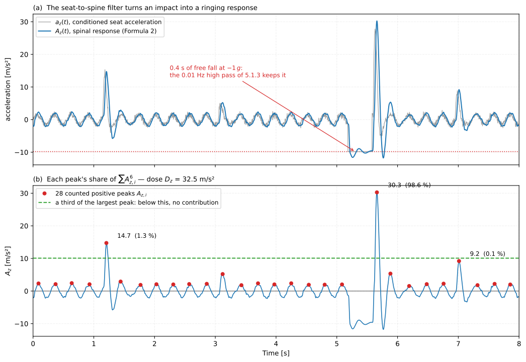

What clause 5 does to a record, in the domain it does it in. The seat-to-spine filter is resonant, so a sharp seat impact becomes a ringing spinal response whose peak arrives later and looks nothing like the input; the zero-crossing rule then counts 28 positive peaks; and the sixth power hands 98.6 % of the dose to one of them. Everything below a third of the largest peak — the dashed line — is contributing hundredths of a percent, which is the rule of clause 5.3 made visible. MultipleShockResult.peaks holds exactly the marked values.

Show the code for this figure

import numpy as np
import matplotlib.pyplot as plt
# `vibration` is the namespace imported in the snippet of section 3.

fs_rec, duration = 256.0, 8.0
time = np.arange(int(duration * fs_rec)) / fs_rec
rng = np.random.default_rng(11)
seat = 1.5 * np.sin(2 * np.pi * 3.6 * time) + 0.45 * rng.standard_normal(time.size)
for start, amplitude in ((1.15, 26.0), (3.05, 8.0), (5.60, 55.0), (6.95, 15.0)):
    hit = time >= start
    seat[hit] += amplitude * np.exp(-20.0 * (time[hit] - start)) * np.sin(
        2 * np.pi * 5.5 * (time[hit] - start))
seat[(time >= 5.18) & (time < 5.58)] = -9.81      # 0.4 s of free fall

response = np.asarray(vibration.spinal_response(seat, fs_rec))
peaks = np.asarray(vibration.response_peaks(response))
shares = 100.0 * peaks**6 / float(np.sum(peaks**6))
print(peaks.size, round(float(peaks.max()), 1), round(float(shares.max()), 1))
# 28 30.3 98.6

fig, (ax_t, ax_p) = plt.subplots(2, 1, sharex=True, figsize=(11, 7.6))
ax_t.plot(time, seat, lw=0.9, color="#9e9e9e", label="$a_z(t)$")
ax_t.plot(time, response, lw=1.5, color="#1f77b4", label="$A_z(t)$")
ax_p.plot(time, response, lw=1.2, color="#1f77b4")
ax_p.axhline(peaks.max() / 3.0, ls="--", color="#2ca02c")
ax_t.legend(loc="upper left")
ax_p.set_xlabel("Time [s]")
plt.show()

5. Injury risk (Annex C)

The daily dose becomes a daily compressive stress $S_d=m_z{D}_{zd}$ (Formula C.1), where $m_z$ (0.029 MPa per m/s² for an 82 kg male, 0.025 for a 64 kg female) converts acceleration to vertebral stress. The stress accumulates over the exposure years against the ageing spine’s reducing ultimate strength $S_u=6.75\mathrm{MPa}-S_{\mathrm{age}}(b+i)$ (Formulae C.3/C.4):

$$R={\left[\sum _{i=0}^{n-1}{\left(\frac{S_d{N}^{1/6}}{S_{u,i}-S_{\mathrm{stat}}}\right)}^6\right]}^{1/6},$$

where $b$ is the age at which the exposure started, $n$ the number of exposure years, $i$ the year counter $0\le i\le n-1$ (so $S_{u,i}$ is the ultimate strength at age $b+i$), and $N$ the number of exposure days per year. $S_{\mathrm{stat}}=m_z\times 9.81m/{\mathrm{s}}^2$ is the static compressive stress the spine already carries under gravity — 0.284 MPa for the male $m_z$, 0.245 MPa for the female one (vibration.static_stress) — and $S_{\mathrm{age}}$ is the annual loss of ultimate strength, 0.052 MPa/year for males and 0.039 MPa/year for females (vibration.ultimate_strength, which returns 5.71 MPa at age 20 and 4.67 MPa at age 40 for a male). The denominator is therefore a margin: $R$ grows both because the dose accumulates day after day and because that margin shrinks by $S_{\mathrm{age}}$ every year, so the same daily dose is more damaging to an older spine.

A Weibull model turns $R$ into the probability of lumbar injury (Formula C.5):

$$\Pi (R)=1-\exp \left[-{\left(\frac{R}{\alpha }\right)}^{\beta }\right].$$

from phonometry import vibration

# Annex C worked example: 5 x 40 m/s2/day, 82 kg male, age 20 for 20 years,
# 120 days/year.
dz = vibration.dose_from_peaks([40.0] * 5)
sd = vibration.compression_dose(dz)                     # 1.62 MPa
r = vibration.injury_risk(sd, start_age=20, years=20, days_per_year=120)
print(round(r, 2))                               # 1.22
print(round(100 * vibration.injury_probability(r)))     # 37  % risk of injury

Reading $R$ (Table C.2)

$R$ has no units and no meaning until it is put on the Table C.2 scale, which gives the value associated with a 10 %, 50 % and 90 % risk of injury for each sex:

Risk of injury	10 %	50 %	90 %
Male	0.72	1.42	2.17
Female	0.52	0.87	1.20

The four bands those thresholds cut out are the ones the fiche of section 6 prints: below the 10 % value a low probability of an adverse health effect, between 10 % and 50 % a moderate one, between 50 % and 90 % a high one, and above the 90 % value a very high one. The male example above, $R$ = 1.22, sits in the moderate band, which is what the standard’s own worked example concludes.

The default matters. compression_dose takes mz and injury_risk takes sex, and both default to the male values. Running the same exposure for a 64 kg female subject does not merely change the number, it changes the verdict:

for sex, mz in (("male", 0.029), ("female", 0.025)):
    sd_sex = vibration.compression_dose(dz, mz=mz)
    r_sex = vibration.injury_risk(sd_sex, start_age=20, years=20,
                                  days_per_year=120, sex=sex)
    print(sex, round(sd_sex, 2), round(r_sex, 2),
          round(100 * float(vibration.injury_probability(r_sex, sex=sex))))
# male   1.62 1.22 37   -> moderate  (10 % < risk < 50 %)
# female 1.40 0.96 64   -> high      (50 % < risk < 90 %)

The lower compressive stress lands in the higher band, because the female thresholds of Table C.2 are lower still. NOTE 5 of Annex C records the same result for this exposure and quotes $R$ = 0.97 against the 0.96 computed here, a rounding of its own printed $S_d$; the band, and therefore the verdict, is the same. The $\alpha$ and $\beta$ coefficients of Formula (C.5) and the Table C.2 thresholds for female subjects rest on a smaller data set, as the standard footnotes both tables.

From a measured time history the whole chain is one call:

import numpy as np
from phonometry import vibration

# A synthetic 10 s seat record at 256 Hz with five 60 m/s2 shocks (stand-in
# for a measured az(t)).
fs = 256.0
az = np.zeros(2560)
az[256::512] = 60.0
result = vibration.multiple_shock_assessment(
    az, fs, start_age=20, years=20, days_per_year=120, sex="male",
    measurement_time=10.0,      # t_m: the record is 10 s long
    exposure_time=4 * 3600.0,   # t_d: 4 h a day in this vehicle
)
print(round(result.acceleration_dose, 2))  # 20.94  m/s2, over the 10 s record
print(round(result.daily_dose, 2))         # 70.35  m/s2, Formula 4 scaled to td
print(round(result.risk, 2))               # 1.53
print(round(result.probability, 2))        # 0.58

result.plot()   # the injury-probability curve with this assessment's R marked (needs matplotlib)

exposure_time and measurement_time are what implement Formula 4 here. Omitted, the measured dose is taken unchanged as the daily dose, which is only correct when the record already covers the whole daily exposure: for this 10 s record and a 4 h day that shortcut divides the dose by $(t_d/t_m{)}^{1/6}=3.36$ and reports $R=0.46$ instead of $1.53$ — a 3 % probability of injury where the exposure gives 58 %.

Show the code for this figure

import numpy as np
import matplotlib.pyplot as plt
from phonometry import vibration

fig, (ax_h, ax_r) = plt.subplots(1, 2, figsize=(12.5, 5.4))

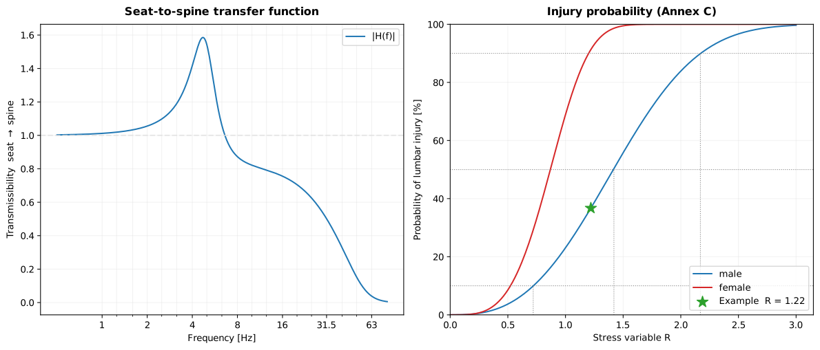
# Left: the seat-to-spine transfer function magnitude (Formula 1).
f = np.logspace(np.log10(0.5), np.log10(80.0), 400)
ax_h.plot(f, np.abs(vibration.seat_to_spine_transfer(f)), label="|H(f)|")
ax_h.set_xscale("log")
ax_h.set_xlabel("Frequency [Hz]")
ax_h.set_ylabel("Transmissibility  seat -> spine")
ax_h.legend()

# Right: the Weibull injury probability for both sexes, with the Annex C
# male example (five 40 m/s2 response peaks a day) marked, which is the R
# the figure prints - not the R of the 10 s synthetic record above.
grid = np.linspace(0.0, 3.0, 300)
for sex in ("male", "female"):
    ax_r.plot(grid, 100.0 * vibration.injury_probability(grid, sex=sex), label=sex)
sd = vibration.compression_dose(vibration.dose_from_peaks([40.0] * 5))
r = vibration.injury_risk(sd, start_age=20, years=20, days_per_year=120)
for level, r_level in zip((10, 50, 90), (0.72, 1.42, 2.17)):  # Table C.2, male
    ax_r.axhline(level, color="#7f7f7f", linestyle=":", lw=0.8)
    ax_r.plot([r_level, r_level], [0.0, level], color="#7f7f7f", linestyle=":", lw=0.8)
ax_r.scatter([r], [100.0 * vibration.injury_probability(r)], marker="*", s=160,
             label=f"Example  R = {r:.2f}")
ax_r.set_xlabel("Stress variable R")
ax_r.set_ylabel("Probability of lumbar injury [%]")
ax_r.legend()
plt.show()

The MultipleShockResult carries the dose $D_z$, the daily dose $D_{zd}$, the compressive stress $S_d$, the stress variable $R$, the injury probability and the response peaks, and its .plot() draws the injury-probability curve with the 10/50/90 % risk thresholds of Table C.2. The model is vertical-axis only: clause 4 neglects the horizontal contributions to spinal compression by design, and the horizontal spinal model of the withdrawn 2004 edition is not reinstated, so horizontal whole-body exposure is assessed instead with the r.m.s., running-r.m.s./MTVV and VDV metrics of Human Vibration (ISO 2631-1).

6. The health-risk report

The dose chain exists to be written down and read against the Annex C guidance. MultipleShockResult.report() writes a one-page PDF health-risk assessment sheet: the standard-basis line (Clause 5 spinal response and the Annex C risk model), an optional metadata header (client, subject, workplace/vehicle, instrumentation, calibration), the exposure-scenario grid (subject sex, the age $b$ at which the exposure started, the number of exposure years $n$, the number of exposure days per year $N$ and the number of counted response shocks), and the dose-and-stress analysis table with the acceleration dose $D_z$ (Formula 3), the daily dose $D_{zd}$ (Formula 4), the daily compressive stress $S_d$ (Formula C.1), the cumulative stress variable $R$ (Formula C.3) and the probability of lumbar injury $\Pi$ (Formula C.5).

Because ISO 2631-5:2018 defines no exposure limit, the fiche carries a risk-band zone row rather than a PASS/FAIL verdict: the boxed $R$ and $\Pi$ name the Annex C risk classification, and a classification table places $R$ among the Table C.2 stress variables for $10$ / $50$ / $90$ % risk of injury (low / moderate / high / very high probability of an adverse health effect), with the injury-probability chart above it. language="es" renders the Spanish fiche (comma decimals).

The metadata argument accepts a ReportMetadata whose relevant fields for a multiple-shock report are client, specimen (the subject), test_room (the workplace or vehicle), test_date, instrumentation, calibration, and the footer identity laboratory, operator, report_id and notes.

import numpy as np
from phonometry import vibration, ReportMetadata

# The Annex C worked example: five 40 m/s2 spinal-response shocks per day,
# 82 kg male, exposed from age 20 for 20 years at 120 days/year. The record is
# rebuilt from those response peaks (the standard states the example in terms
# of the peaks), so the fiche prints the published Annex C values. The five
# peaks are the whole day, so td = tm and daily_dose is dz unscaled.
peaks = np.array([40.0] * 5)
dz = vibration.dose_from_peaks(peaks)
sd = vibration.compression_dose(dz)
r = vibration.injury_risk(sd, start_age=20, years=20, days_per_year=120)
result = vibration.MultipleShockResult(
    sex="male",
    acceleration_dose=dz,
    daily_dose=dz,
    compression_dose=sd,
    risk=r,
    probability=float(vibration.injury_probability(r)),
    start_age=20.0,
    years=20,
    days_per_year=120.0,
    peaks=peaks,
    risk_thresholds=(0.72, 1.42, 2.17),   # Table C.2, male: 10 / 50 / 90 % risk
)

result.report(
    "multiple_shock.pdf",
    metadata=ReportMetadata(
        client="Example transport operator",
        specimen="82 kg male operator (seated)",
        test_room="Off-road vehicle, driver's seat",
        report_id="EXAMPLE-2631-5",
    ),
)   # R = 1.22, Pi = 37 % -> moderate probability of an adverse health effect

The example fiche is regenerated with make reports and kept rendered in the repository; click the preview to open the PDF.

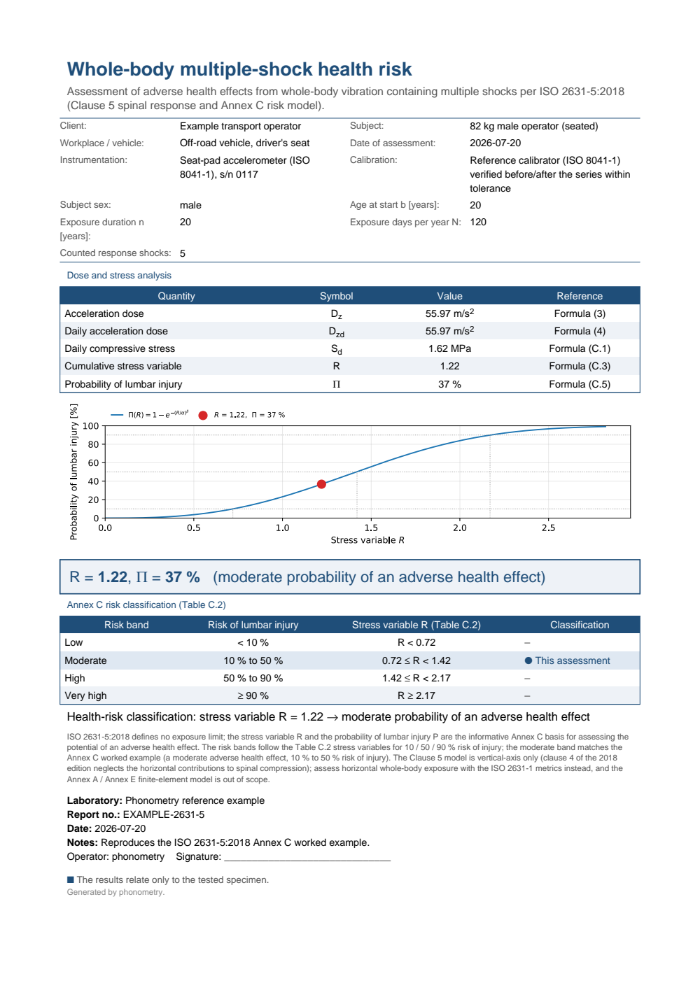
One-page whole-body multiple-shock health-risk assessment fiche: a header with the transport operator, the subject and the off-road vehicle, the exposure-scenario grid (82 kg male, age 20, 20 years, 120 days per year, five counted shocks), the dose-and-stress analysis table with the acceleration dose Dz = 55.97 m/s2, the daily compressive stress Sd = 1.62 MPa, the cumulative stress variable R = 1.22 and the probability of lumbar injury 37 percent, the injury-probability curve with the Table C.2 risk levels and this assessment marked, the boxed R = 1.22 and 37 percent classed as a moderate probability of an adverse health effect, and the Annex C classification table where the moderate band (10 to 50 percent risk of injury) is the assessment's band.

Download the report (PDF)

Whole-body multiple-shock health-risk fiche (MultipleShockResult.report), the ISO 2631-5:2018 Annex C worked example with the dose-and-stress analysis and the Table C.2 risk classification.

What this guide covers

• Covered

  ISO 2631-5:2018 clause 5 and Annex C. The acquisition and conditioning requirements of clauses 5.1.2 to 5.1.4 as guidance; the clause 5.2 seat-to-spine transfer function (seat_to_spine_transfer, spinal_response, response_peaks); the clause 5.3 acceleration dose and the Formula 4 daily dose (dose_from_peaks, acceleration_dose, daily_dose, and the measurement_time / exposure_time pair of multiple_shock_assessment); and the Annex C compressive stress, cumulative stress variable and Weibull probability with their Table C.1 coefficients and Table C.2 thresholds (compression_dose, static_stress, ultimate_strength, injury_risk, injury_probability, multiple_shock_assessment, MultipleShockResult.report).

• Not covered

  The Annex A / Annex E finite-element model for the less severe exposures of clause 4 — occupants who stay seated throughout, which is most agricultural and earth-moving work — is distributed by ISO as separate software and is not implemented here; a record from that regime has no route through this page. Neither is the horizontal spinal model of the withdrawn 2004 edition, so horizontal whole-body exposure goes to the r.m.s., running-r.m.s./MTVV and VDV metrics of Human Vibration. The conditioning chain of section 2 is the caller’s: spinal_response assumes a record that has already been sign-checked, split at the loss-of-contact boundaries, offset-corrected, tapered and band-limited.

See also

• Human Vibration: the ISO 2631-1 chain this page hands back to for the horizontal axes, and the crest factor and clause 6.3.3 ratios that decide whether a record belongs here at all.
• API reference: vibration.human.multiple_shock.
• Theory: Multiple shocks (ISO 2631-5): the ISO 2631-5 response model, the acceleration dose and the Weibull risk law.

References

• Griffin, M. J. (1996). Handbook of human vibration. Academic Press. ISBN 978-0-12-303041-2. Background on whole-body shock exposure, spinal biodynamics and the lumbar health effects that the ISO 2631-5 dose model quantifies.
• International Organization for Standardization. (2016). Mechanical vibration — Laboratory method for evaluating vehicle seat vibration — Part 1: Basic requirements (ISO 10326-1:2016). The accelerometer disc on the seat pad that clause 5.1.2 requires: its diameter, height and hardness, and the metal disc that carries the transducers (5.2.3).
• International Organization for Standardization. (2018). Mechanical vibration and shock — Evaluation of human exposure to whole-body vibration — Part 5: Method for evaluation of vibration containing multiple shocks (ISO 2631-5:2018). The acquisition and conditioning of the record (clauses 5.1.2 to 5.1.4), the seat-to-spine transfer function (clause 5.2, Formula 1), the acceleration and daily dose (clause 5.3, Formulae 3-5) and the Annex C assessment of adverse health effects (Formulae C.1, C.3-C.5, Tables C.1/C.2).