Measuring vibration immission (DIN 45669-1)
Standards: DIN 45669DIN 45669-1 Ber 1DIN 4150
German immission control judges vibration in buildings with two standards that print thresholds and say almost nothing about how the number reaching them was formed. DIN 4150-2 sets what people in buildings may be exposed to and DIN 4150-3 sets what the buildings themselves may take. Both are tables of values for a quantity that has to come from somewhere, and DIN 45669-1 is where it comes from: the specification of the vibration meter, which is also the definition of the quantities those tables compare against.
That makes this page the other half of a pair. The damage page reads a guideline value off a table; this one builds the number you read it with, from a velocity record, and then grades an instrument that claims to produce it. The two standards meet twice: once because the meter is what a DIN 4150 measurement is made with, and once in Annex E, where the guideline curve of DIN 4150-3 comes back as a filter.
1. The chain, in the order the standard builds it
Section titled “1. The chain, in the order the standard builds it”A velocity signal enters and four numbers come out. Between them are three stages, each printed as an exact transfer function or an exact average.
Band limitation (5.2.3.2, Formula (3)) is two Butterworth pairs: a
two-pole high pass at 0,8 f_u and a two-pole low pass at f_o / 0,8. The
working range is 1 Hz to 80 Hz for buildings, so those corners are 0,8 Hz and
100 Hz. Next to a railway the range is 4 Hz to 315 Hz, which is where
DIN 45672 works, and
blasting and structure-borne sound need it too.
Frequency weighting (Formula (4)) divides that by
1 − j 5,6 Hz / f, one more pole and one more zero. Normalising the result by
1 mm/s turns it into the KB signal, which is dimensionless and is what
everything downstream is built on.
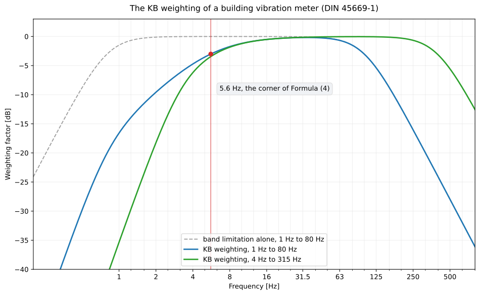
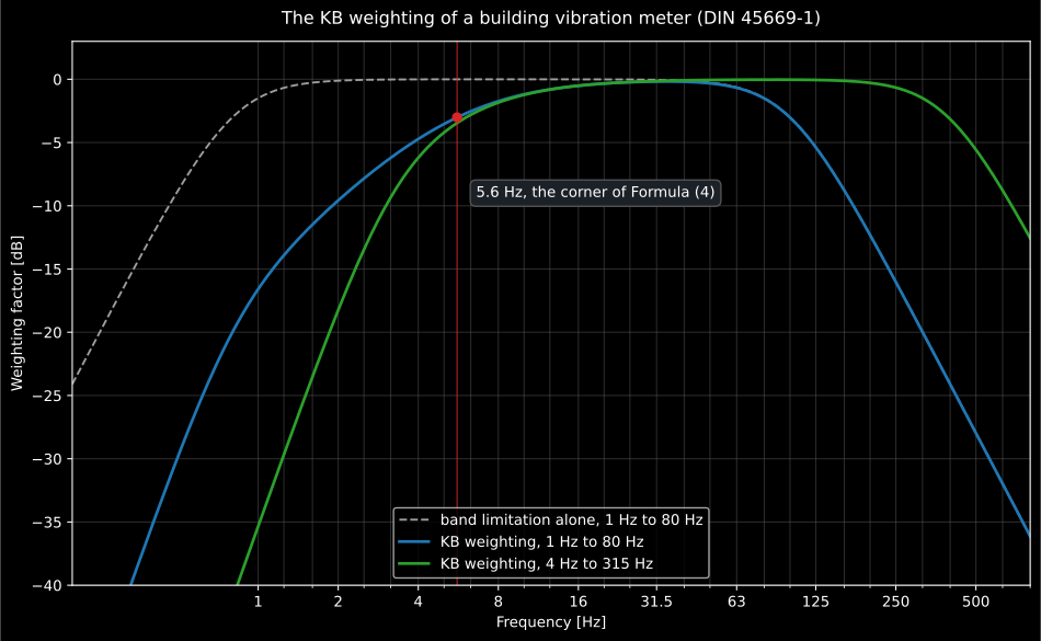
Figure code
import matplotlib.pyplot as pltimport numpy as np
from phonometry import vibration
freqs = np.geomspace(0.2, 800.0, 600)building = np.abs(vibration.kb_weighting_response(freqs))railway = np.abs(vibration.kb_weighting_response(freqs, working_range="railway"))band = np.abs(vibration.band_limitation_response(freqs))
fig, ax = plt.subplots(figsize=(10, 6.2))ax.semilogx(freqs, 20 * np.log10(band), "--", label="band limitation alone")ax.semilogx(freqs, 20 * np.log10(building), label="KB weighting, 1 Hz to 80 Hz")ax.semilogx(freqs, 20 * np.log10(railway), label="KB weighting, 4 Hz to 315 Hz")ax.axvline(vibration.KB_CORNER_HZ)ax.set_xlabel("Frequency [Hz]")ax.set_ylabel("Weighting factor [dB]")ax.set_ylim(-40, 3)ax.legend()
The magnitudes of both are printed as Formulae (5) and (6), and the library returns the complex responses so a phase check has something to read:
import numpy as np
from phonometry import vibration
kb = np.abs(vibration.kb_weighting_response([16.0]))print(f"KB weighting at the reference frequency: {kb[0]:.4f}")  # 0.9435
corners = np.abs(vibration.band_limitation_response([0.8, 100.0]))print(f"the two band-limit corners: {corners.round(4)}")  # [0.7071 0.7071]
2. What a meter displays, and the two rules inside Formula (2)
Section titled “2. What a meter displays, and the two rules inside Formula (2)”The KB signal is averaged, and the averaging is the one a sound level meter
calls Fast: a running r.m.s. with τ = 0,125 s (Formula (1)). Its value at any
instant is the weighted vibration severity KB_F(t), and 3.10.1.2 says
why that time constant: DIN 4150-2 judges the effect on people with it, and
the fluctuating indication it gives below 5 Hz was taken into account when
those judging criteria were written.
From that signal come the three numbers a measurement is reported as. The
maximum KB_Fmax over the averaging time. The maximum inside each clock
interval (Takt) of 30 s, which DIN 4150-2 fixes. And the r.m.s. of those
clock maxima, KB_FTm, from Formula (2), which carries two rules that are
easy to read past:
- a clock maximum at or below 0,1 enters the sum as zero, and the interval it came from still counts in N, so a quiet stretch pulls the average down rather than being dropped from it;
- a clock interval the measurement did not fill is not a clock interval (5.1.6.4), so the averaging time always spans a whole number of them.
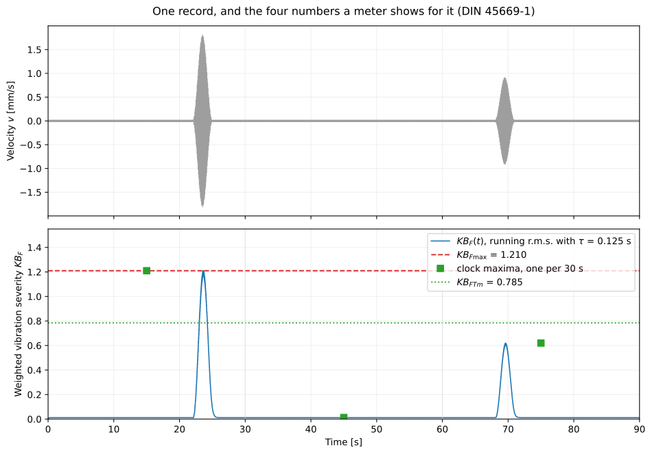
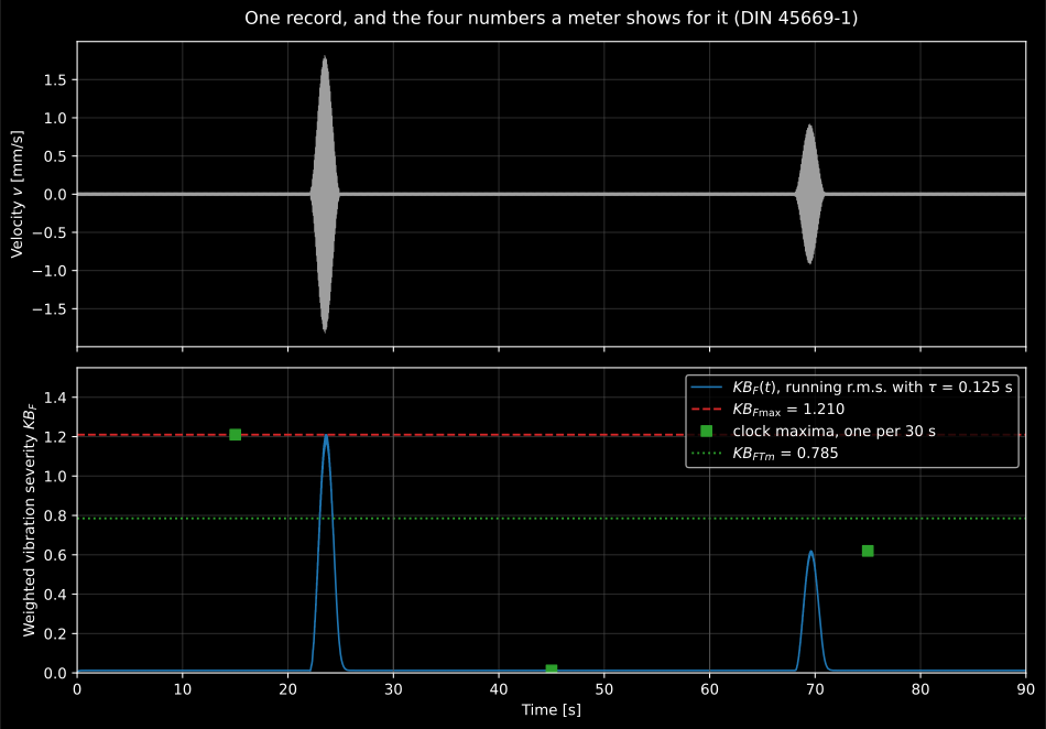
Figure code
import matplotlib.pyplot as pltimport numpy as np
from phonometry import vibration
fs_hz = 2048.0t = np.arange(int(90.0 * fs_hz)) / fs_hzrecord = 0.02 * np.sin(2 * np.pi * 11.0 * t)for start, amplitude, frequency in ((22.0, 1.8, 17.0), (68.0, 0.9, 26.0)):    window = (t >= start) & (t < start + 3.0)    record[window] += (        amplitude        * np.hanning(int(window.sum()))        * np.sin(2 * np.pi * frequency * t[window])    )
reading = vibration.measure_vibration_immission(record, fs_hz)reading.plot()
The record above is one that a real measurement looks like: a machine running somewhere nearby, and two events. Running it through the chain gives the four numbers, and the third clock interval is where Formula (2) shows its teeth.
import numpy as np
from phonometry import vibration
fs_hz = 2048.0t = np.arange(int(90.0 * fs_hz)) / fs_hzrecord = 0.02 * np.sin(2 * np.pi * 11.0 * t)for start, amplitude, frequency in ((22.0, 1.8, 17.0), (68.0, 0.9, 26.0)):    window = (t >= start) & (t < start + 3.0)    record[window] += (        amplitude        * np.hanning(int(window.sum()))        * np.sin(2 * np.pi * frequency * t[window])    )
reading = vibration.measure_vibration_immission(record, fs_hz)print(f"|v|max      = {reading.peak_velocity_mm_s:.3f} mm/s")  # 1.816 mm/sprint(f"KB_Fmax     = {reading.kbf_max:.3f}")                  # 1.210print(f"clock maxima= {reading.takt_maxima.round(3)}")         # [1.21 0.013 0.62]print(f"KB_FTm      = {reading.kbf_takt_rms:.3f}")             # 0.785
quiet = reading.takt_maxima[1]counted = np.array([reading.takt_maxima[0], 0.0, reading.takt_maxima[2]])print(f"the quiet interval reads {quiet:.3f}, enters as 0, and still counts:")print(f"  sqrt(mean of squares over 3) = {np.sqrt(np.mean(counted**2)):.3f}")
Start the record before the event. Every filter here begins at rest, so a record that begins with the signal already at full amplitude carries the filter’s own switch-on transient, and the peak is a max-hold that keeps it. A 1 mm/s sine started at a zero crossing reads 1,06 mm/s rather than the 1,00 mm/s of 6.2.3.12. That is a property of the record, not of the chain, and a second of quiet in front of the event removes it.
3. The numbers the standard prints for a meter to reproduce
Section titled “3. The numbers the standard prints for a meter to reproduce”Two tables make the chain checkable rather than merely specified. Table 9 (on printed folio 35) says what a 1 mm/s sine has to show at five frequencies, and Table 8, in the redraft Corrigendum 1 gives it, says the same for a burst train. They are published here as data, and the conformance report runs them:
from phonometry import vibration
for frequency_hz, (kbf, kbf_max, kbf_takt) in vibration.KB_TEST_INDICATIONS.items():    print(f"{frequency_hz:6.1f} Hz -> KB_F {kbf:.3f}, KB_Fmax {kbf_max:.3f}")
print(vibration.KB_REFERENCE_INDICATIONS)# {'peak_velocity_mm_s': 1.0, 'kbf': 0.667, 'kbf_max': 0.68, 'kbf_takt_rms': 0.68}
KB_Fmax above KB_F in every row is not a gain: it is the ripple of a
running r.m.s. of a sine, which Annex B is about, and it is why these values
are worth having as an oracle. No closed form for the pair is printed
anywhere, so a check that reproduces them checks the whole chain, filter,
squaring, averaging and maximum together.
4. Grading a meter: Tables 2 and 3
Section titled “4. Grading a meter: Tables 2 and 3”The tolerance is not on the response but on its shape. Formula (7) divides
the measured response by the design response, each normalised at the reference
frequency of 16 Hz, so a flat gain error is a calibration matter and not a
conformity one. What is left is graded band by band: 10 % from 1,25 f_u to
0,8 f_o, 20 % out to 0,5 f_u and 2 f_o, and below that Table 2 stops
constraining the response from below altogether.
import numpy as np
from phonometry import vibration
frequencies_hz = np.array([1.0, 2.0, 4.0, 8.0, 16.0, 31.5, 63.0, 80.0])measured = np.abs(vibration.kb_weighting_response(frequencies_hz))measured[5] *= 1.15  # a meter 15 % high at 31,5 Hz
result = vibration.verify_vibration_meter(frequencies_hz, measured)print(f"passes: {result.passes}")                       # Falseprint(f"worst frequency: {result.worst_frequency_hz} Hz")  # 31.5 Hz
The reference frequency itself carries no requirement, the standard writing every limit “for all f not equal to f_r”, so it is dropped from the verdict rather than passed for free. And a verdict here is one clause: Clause 6 also asks for linearity, overload, crest-factor handling, temperature, humidity and electromagnetic tests, all of them measurements on hardware.
5. Annex E: judging a building without a dominant frequency
Section titled “5. Annex E: judging a building without a dominant frequency”DIN 4150-3 compares a peak velocity with a guideline value that depends on frequency, which means a short-term event has to be given one. Annex D gives two ways of finding it, the zero crossings around the largest amplitude and the Fourier transform of the whole event, and says plainly that they can disagree. They do:
import numpy as np
from phonometry import vibration
fs_hz = 2048.0t = np.arange(int(3.0 * fs_hz)) / fs_hzevent = np.sin(2 * np.pi * 17.0 * t) * np.hanning(t.size)
print(vibration.dominant_frequency(event, fs_hz).frequency_hz)  # 17.07 Hzprint(vibration.dominant_frequency(event, fs_hz, method="fourier").frequency_hz)
The disagreement matters because the frequency picks the guideline value, so
it can change the verdict. Annex E removes the question instead of refining
it. Each building class of DIN 4150-3 Table 1 gets a weighting filter
whose target magnitude is that class’s guideline curve inverted and normalised
to the value it holds from 1 Hz to 10 Hz. Filter the velocity with it and the
peak of what comes out, the assessment velocity v_Bn, is compared with a
single number that no longer depends on frequency: 20, 5 or 3 mm/s (Table E.2).
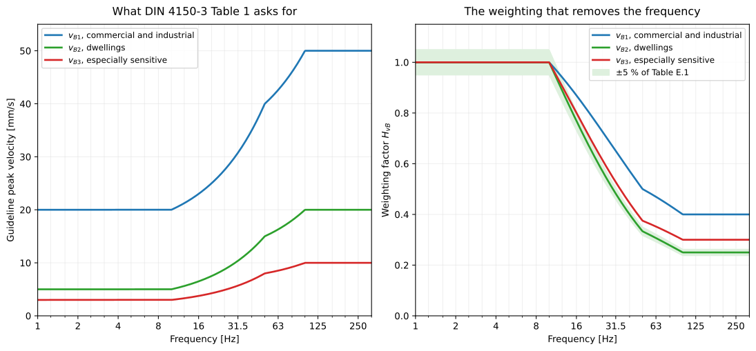
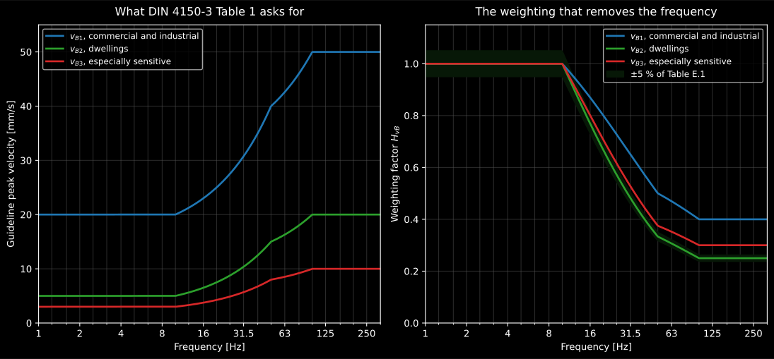
Figure code
import matplotlib.pyplot as pltimport numpy as np
from phonometry import vibration
freqs = np.geomspace(1.0, 315.0, 500)fig, axes = plt.subplots(1, 2, figsize=(11.5, 5.4))for cls in vibration.ASSESSMENT_GUIDE_VALUES_MM_S:    axes[0].plot(freqs, vibration.guideline_velocity(cls, freqs), label=cls)    axes[1].plot(        freqs,        vibration.assessment_weighting_response(freqs, building_class=cls),        label=cls,    )for ax in axes:    ax.set_xscale("log")    ax.set_xlabel("Frequency [Hz]")    ax.legend()
The filter is specified as a target magnitude with a ±5 % band and a linear phase, and the annex says why the phase: a weighting that delays different frequencies differently changes the peak it is there to measure. A symmetric FIR is the type it names, and the library designs one.
The two routes agree, which is the point of the annex:
import numpy as np
from phonometry import vibration
fs_hz = 2048.0t = np.arange(int(3.0 * fs_hz)) / fs_hzevent = 1.8 * np.sin(2 * np.pi * 17.0 * t) * np.hanning(t.size)
# The DIN 4150-3 route: find the frequency, read the guideline value there.peak_mm_s = float(np.max(np.abs(event)))guideline = float(vibration.guideline_velocity("residential", 17.0))print(f"peak {peak_mm_s:.3f} mm/s against {guideline:.2f} mm/s at 17 Hz")print(f"  ratio {peak_mm_s / guideline:.3f}")  # 0.269
# The Annex E route: no frequency anywhere.assessment = vibration.assess_short_term_vibration(    event, fs_hz, building_class="residential")print(f"|v_B2|max {assessment.assessment_velocity_mm_s:.3f} mm/s against 5 mm/s")print(f"  ratio {assessment.ratio:.3f}")  # 0.271print(f"  within the guideline: {assessment.within_guideline}")
The verdict reads the way DIN 4150-3 reads: keeping to the value is what the standard has evidence about, and exceeding it does not mean damage has occurred, only that the cheap check has run out and Clauses 4.2 to 4.4 have to be done instead.
6. Setting the transducer down: what DIN 45669-2 puts a number to
Section titled “6. Setting the transducer down: what DIN 45669-2 puts a number to”DIN 45669 has a second part, and it is the one a measurement is actually planned with: DIN 45669-2 fixes where the transducers go, how they are coupled to a floor or to the ground, how long a measurement runs and which disturbances have to be kept out of it. Nearly all of it is judgement written down. The little that is a number is here, because a number a measurement is planned by belongs where the plan is checked.
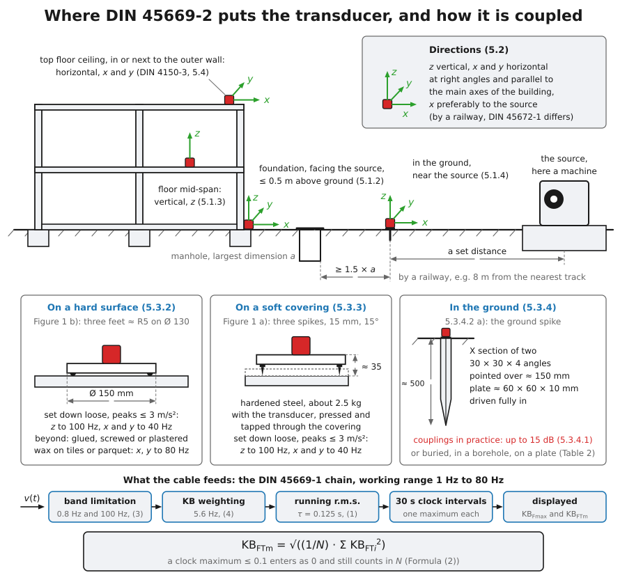
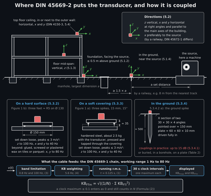
A transducer set down without fastening walks or lifts off when the vibration is strong, and a coupling that is not force-locked resonates against the surface. Clauses 5.3.2 and 5.3.3 fix both limits: a loose transducer measures without falsification up to 100 Hz vertically and 40 Hz horizontally, provided the peak acceleration in every direction stays at or below 3 m/s². On a hard surface it may stand on its own or on the device with rounded feet; on a carpet it has to stand on the device with hardened steel spikes, about 2,5 kg with the transducer, pressed and tapped through the covering. Above those limits the transducer is glued, screwed or plastered on, and on tiles or parquet adhesive wax carries the horizontal component to 80 Hz.
from phonometry import vibration
floor = vibration.check_loose_mounting(1.2, 63.0, direction="horizontal")print(f"loose, horizontal to 63 Hz: {floor.acceptable}")  # Falseprint(f"  limit {floor.frequency_limit_hz:g} Hz, {floor.peak_acceleration_limit_m_s2:g} m/s2")
carpet = vibration.check_loose_mounting(    1.2, 80.0, direction="vertical", surface="soft")print(f"loose, vertical to 80 Hz on a carpet: {carpet.acceptable}")  # Trueprint(f"  on {carpet.device}")
Two more numbers belong to the plan. The mass the transducer and its device
add to the object should be at most a hundredth of the mass the object
vibrates with (7.2.4), and mass_loading_ratio is that fraction. And Table 3
says how far a meter that meets every requirement of DIN 45669-1 may still be
from the truth on one displayed quantity: 15 % on a value based on an r.m.s.
and 20 % on a peak, at a high confidence level. The table prints a second
column for a class 2 meter; the 2010 edition of Part 1 dropped the accuracy
classes, so the first column is the one a meter of today is held to.
from phonometry import vibration
print(vibration.instrument_confidence_limit_percent("rms"))   # 15.0print(vibration.instrument_confidence_limit_percent("peak"))  # 20.0print(f"{vibration.mass_loading_ratio(2.5, vibrating_mass_kg=600.0):.4f}")  # 0.0042print(vibration.MASS_LOADING_RATIO_LIMIT)  # 0.01
The coupling to the ground has no such number, only a warning: 5.3.4.1 says that the coupling alone can move the reading by up to 15 dB, and that the horizontal components suffer most. Which of the four methods of Table 2 to use is the one judgement Part 2 leaves entirely to the reader.
How the measurement goes
Section titled “How the measurement goes”Use a meter that meets DIN 45669-1, with three channels so the three directions are recorded together, and a fourth near the source when its signal must be told apart from the rest. On site, run at least one check of the chain once the meter has had the warm-up time its maker states: a vibration calibrator, a tap test, or an electrical signal fed to the input and read against the reference indications, the last always together with one of the other checks; if the electrical check is more than 10 % off, find out why.
Choose the positions by the question: for the building, the foundation nearest
the source, no higher than 0,5 m above ground, and the top floor ceiling next
to the outer wall; for its occupants, their floors at mid-span; for a building
still to be built, the ground of the plot it will stand on; to find what the
source itself emits, the ground near it at a set distance, at least 1,5 times
the largest dimension of a manhole or other disturbing body away from that
body. Point z up and x and y along the main axes of the building, x
preferably towards the source. Couple the transducer as the insets show, keep
it and its device to at most a hundredth of the mass vibrating with the
object, and lay low-noise coaxial cable that cannot move against the object.
Measure over the whole assessment time or stretches that represent it; DIN 4150-2 assesses people over 16 h by day and 8 h by night. DIN 45669-2 prints no background correction: judge vibration from other sources, where you can, by comparing the indications with and without the source running, helped by a frequency analysis or the channel near the source. Report the purpose, the instruments, the positions on a site plan, the directions, the coupling, the times, the source, the results, the disturbances and what could be felt or heard rattling.
7. What this page is not
Section titled “7. What this page is not”Measurement positions, directions, durations and the list of disturbances are the text of DIN 45669-2: section 6 describes them, and none of it is computed here. What is here is the instrument the two parts describe between them, the quantities it is required to produce, and the limits a measurement with it is planned by.
The band limitation of Formula (3) and the KB weighting of Formula (4), complex, over both working ranges of 5.2.3.1, with the magnitudes of Formulae (5) and (6) as their absolute values.
The weighted vibration severity
KB_F(t)of Formula (1), its maximum, the clock maxima of the 30 s intervals of 5.1.6.4 and the clock maximum r.m.s. of Formula (2), including its two counting rules, and the detection limits of 5.2.2.The amplitude response tolerances of Tables 2 and 3 with the deviation of Formula (7), as a verdict on a measured response; and the printed check values of Table 9, of 6.2.3.12 and of Table 8 in the redraft of Corrigendum 1, reproduced by running the chain.
Annex E in full: the three assessment weightings of Table E.1 as a target magnitude and as a linear-phase FIR, the assessment velocity they produce and the frequency-independent guideline values of Table E.2. And Annex D, both methods of finding a dominant frequency.
Not covered
No bench. Clause 6 also grades linearity, overload, crest-factor handling, the digital interfaces, temperature, humidity and electromagnetic susceptibility. Those are measurements on hardware and a pass on the response is not a conformity certificate for an instrument.
The numbers of DIN 45669-2: the loose-mounting limits of 5.3.2 and 5.3.3 as a verdict, the wax limit of Table 1, the mass loading of 7.2.4 and the instrument confidence limits of Table 3.
No measurement procedure in code. Measurement positions, directions, durations, the choice of a ground coupling and the treatment of disturbances are the text of DIN 45669-2, described in section 6 and not computed, and the assessment of what was measured is DIN 4150-2 and DIN 4150-3.
What this guide covers
Section titled “What this guide covers”References
Section titled “References”- Deutsches Institut für Normung. (1999). Erschütterungen im Bauwesen — Teil 3: Einwirkungen auf bauliche Anlagen (DIN 4150-3:1999-02). Table 1, whose guideline curve the Annex E weightings invert, the three building classes they are written for, and the measuring points of 5.4.
- Deutsches Institut für Normung. (2005). Messung von Schwingungsimmissionen — Teil 2: Messverfahren (DIN 45669-2:2005-06). The loose-mounting limits of 5.3.2 and 5.3.3, the wax limit of Table 1, the mass loading of 7.2.4, the ground coupling deviation of 5.3.4.1 and the confidence limits of Table 3. Measurement positions, directions, durations, the choice of a ground coupling and disturbances are text and are not implemented.
- Deutsches Institut für Normung. (2010). Messung von Schwingungsimmissionen — Teil 1: Schwingungsmesser — Anforderungen und Prüfungen (DIN 45669-1:2010-09). The working ranges of 5.2.3.1, the band limitation and frequency weighting of Formulae (3) to (6), the running r.m.s. of Formula (1) and the clock maximum r.m.s. of Formula (2), the display quantities of 5.1.6, the detection limits of 5.2.2, the amplitude response tolerances of Tables 2 and 3 with the deviation of Formula (7), the reference conditions of 5.2.10 and the reference indications of 6.2.3.12 with Table 9, the dominant frequency methods of Annex D, the assessment weightings and guideline values of Annex E with Tables E.1 and E.2, and the channel count of 5.1.2 and the on-site checks of 6.5. The design and type-test clauses that need a bench are not implemented.
- Deutsches Institut für Normung. (2012). Messung von Schwingungsimmissionen — Teil 1: Schwingungsmesser — Anforderungen und Prüfungen, Berichtigung 1 (DIN 45669-1 Ber 1:2012-12). The redraft of Table 8, the eight burst durations of an 80 Hz signal and the KB_Fmax each must show as a percentage of the continuous indication.