Machine fault frequencies

Condition monitoring begins with arithmetic, not with signal processing. Every rolling-contact bearing, gear pair, induction motor and bladed rotor excites a family of discrete frequencies fixed by its geometry and its shaft speed, and knowing where those lines fall is what turns a featureless spectrum into a diagnosis: a peak is only evidence when it sits on a named line. This page covers the kinematics of M. P. Norton and D. G. Karczub, Fundamentals of Noise and Vibration Analysis for Engineers (2nd ed., Cambridge University Press, 2003), Section 8.4, and how they combine with the signal chain the library already provides - the envelope spectrum and cepstrum and time synchronous averaging.

The working view is the two put together: the envelope spectrum of a band-passed vibration record with the predicted lines drawn on top and named.

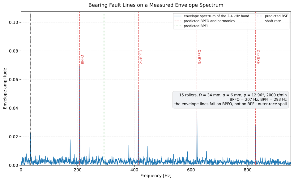
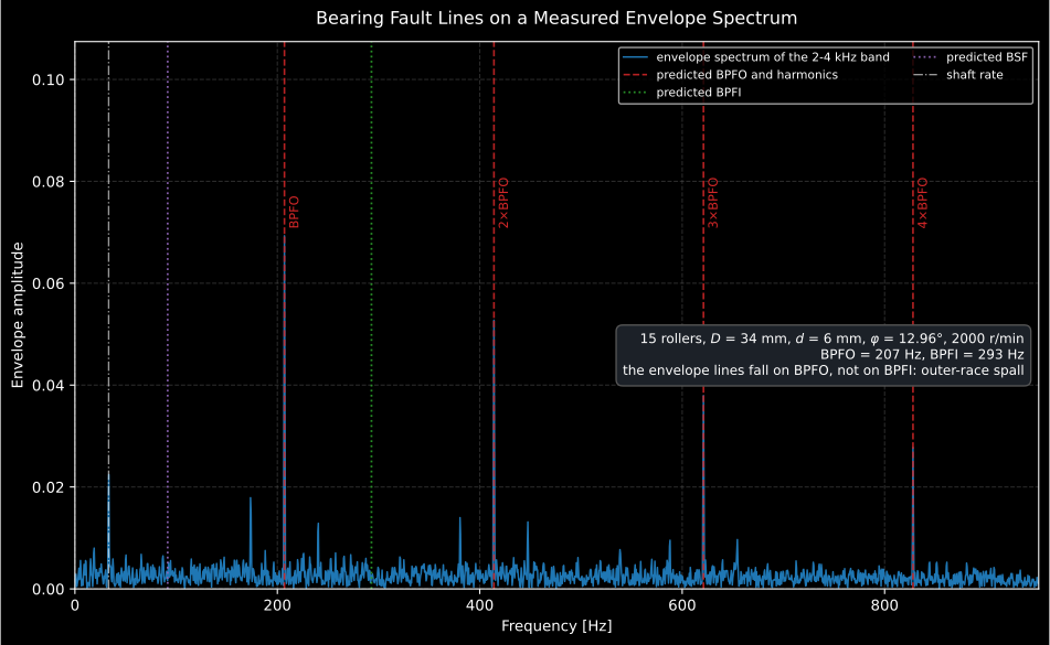
The four tall lines land on BPFO and its harmonics; nothing appears on BPFI, on the roller rate BSF or on the 183 Hz BDF where a damaged roller would strike. That is the diagnosis: a spall on the outer race.

Show the code for this figure

import matplotlib.pyplot as plt
import numpy as np
from phonometry import bearing_fault_frequencies, envelope_spectrum, noise_signal

# The bearing: 15 rollers on a 34 mm pitch diameter, 6 mm rollers,
# 12.96 degrees contact angle, shaft at 2000 r/min.
faults = bearing_fault_frequencies(2000.0, 15, 6.0, 34.0,
                                   contact_angle_deg=12.96)
bpfo, shaft = faults["BPFO"], faults.shaft_rate    # 207.0 Hz, 33.33 Hz

# A spalled outer race: one impact per BPFO period, each ringing a 3 kHz
# housing resonance, load-modulated once per revolution, buried in noise.
fs, seconds = 20000.0, 2.0
t = np.arange(int(fs * seconds)) / fs
impacts = np.zeros_like(t)
for k in range(int(seconds * bpfo)):
    impacts[round(k / bpfo * fs)] = 1.0 + 0.35 * np.cos(
        2.0 * np.pi * shaft * k / bpfo)
tau = np.arange(int(0.004 * fs)) / fs
ring = np.exp(-tau / 6.0e-4) * np.sin(2.0 * np.pi * 3000.0 * tau)
x = np.convolve(impacts, ring)[: t.size] * 0.6
x += 0.35 * np.sin(2.0 * np.pi * shaft * t)          # residual unbalance
x += noise_signal(fs, seconds, color="white", rms=0.25, seed=17)

# Band-pass the resonance the impacts ring, envelope it, transform it,
# and let the result draw its own lines on top.
spectrum = envelope_spectrum(x, fs, band=(2000.0, 4000.0))
faults.within(1.0, 5.0 * bpfo).plot(spectrum=spectrum)
plt.show()

Symbols on this page

Norton keeps the notation of his sources, and one letter carries four different meanings across the four sections. The table below is the key; the one to watch is $N$, which is a speed in section 1 and a count in sections 2 and 4.

Symbol	Meaning	Unit	Section
$N$	shaft speed (the API’s first positional argument)	r/min	1
$f_s$	shaft rotational frequency, $f_s=N/60$	Hz	all
$Z$	number of rolling elements in the bearing	—	1
$d$, $D$	rolling-element diameter, pitch diameter	same unit for both	1
$\varphi$	contact angle, from the radial plane	degrees	1
$g$	the shared factor $g=(d/D)\cos \varphi$	—	1
$N$	number of gear teeth on the wheel (Norton’s Eq. 8.3)	—	2
$R$, $p$	rotor bars, magnetic poles (not pole pairs)	—	3
$s$, $f_e$	slip (a fraction, not a percentage), supply frequency	—, Hz	3
$N$, $V$	number of rotor blades, number of stator vanes	—	4
$N$	number of pumping events per revolution	—	4
$n$	harmonic index (rotor-slot in section 3, blade in section 4)	—	3, 4
$m_L$	number of lobes of a rotating interaction pattern	—	4

Nothing in the library reuses the name: bearing_fault_frequencies, gear_mesh_frequencies and blade_pass_frequencies all take the shaft speed in r/min first and the count second, so the collision lives in the printed formulae only. It is still worth checking, because a count substituted for a speed is a factor-of-60 error that raises no exception.

1. Rolling-contact bearings

Norton reproduces the eleven equations collected by Shahan and Kamperman (Eqs. 8.4 to 8.14). They collapse to seven distinct frequencies, because four of the eleven are the rotating-inner-race counterparts of rows already in the table — either pairwise identical to them or reached through the rotating_race argument. With the shaft speed $N$ in r/min, $Z$ rolling elements of diameter $d$ on a pitch diameter $D$, a contact angle $\varphi$, and writing $g=(d/D)\cos \varphi$ and $f_s=N/60$:

Name	Meaning	Expression	Norton eq.
shaft	shaft rotational frequency	$f_s=N/60$	(8.4)
FTF	cage (fundamental train) frequency	$(f_s/2)(1-g)$	(8.5)
FTF_rel	cage relative to the rotating race	$f_s-\text{FTF}$	(8.11)
BSF	rolling-element rotational frequency	$(f_s/2)(D/d)(1-g^2)$	(8.7)
BDF	rolling-element spin frequency	$2\text{BSF}$	(8.10)
BPFO	element pass frequency, outer race	$Z(f_s/2)(1-g)$	(8.8)
BPFI	element pass frequency, inner race	$Z(f_s/2)(1+g)$	(8.9)

Those three geometric quantities carry the whole family, and two of them are routinely mistaken. The pitch diameter is measured between the rolling-element centres, not across the bore and not across the outside diameter. The contact angle is measured from the radial plane, so it does not appear in an end view at all: it is zero for a deep-groove ball bearing and non-zero for angular-contact and tapered-roller types, which is the only reason $g=(d/D)\cos \varphi$ has a cosine in it.

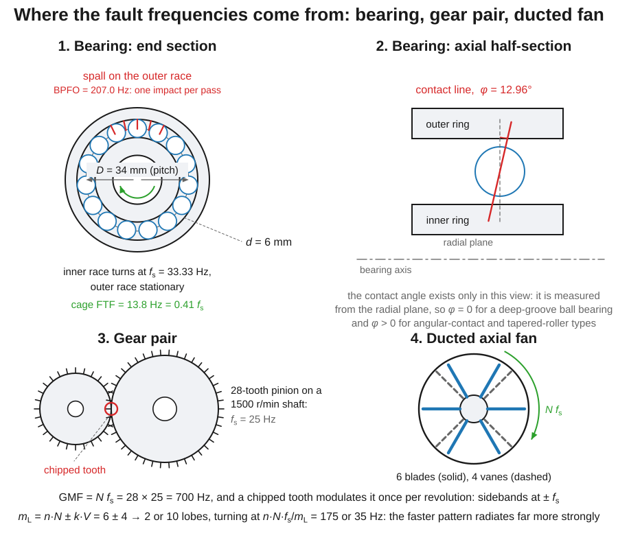
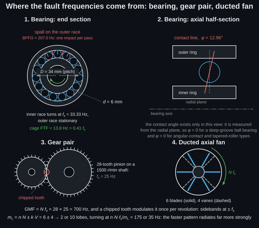
The two exact identities the section leans on are geometric statements this picture makes obvious: every element passes either the outer-race defect or the inner-race one, so $\text{BPFO}+\text{BPFI}=Z{f}_s$; and with a stationary outer race the cage carries all $Z$ elements past the defect once per cage revolution, so $\text{BPFO}=Z\times \text{FTF}$.

Three of them carry the diagnosis: BPFO for an outer-race defect, BPFI for an inner-race defect, and BDF for a damaged rolling element or cage. The two rolling-element rows are one factor of two apart because they answer different questions: BSF is how fast a roller turns, BDF how often a defect on it strikes a race — twice per roller revolution, once against each. Evidence of a damaged roller is therefore expected at BDF (183.3 Hz for the bearing above), usually modulated at the cage rate FTF, while the line the figure draws at 91.7 Hz is the roller’s rotational rate BSF. Two identities are worth remembering because they are exact and catch data-entry errors instantly: $\text{BPFO}+\text{BPFI}=Z{f}_s$ always, and $\text{BPFO}=Z\times \text{FTF}$ whenever the outer race is stationary.

Presence and absence is the weak form of the diagnosis, and it works here only because this bearing’s BPFO (207 Hz) and BPFI (293 Hz) are far apart and the record is clean. The strong form is the modulation, and it follows from the same geometry:

• an outer-race defect sits at a fixed angular position in the load zone, so every rolling element strikes it under the same load. The impact train is unmodulated, and BPFO appears as a clean harmonic series with little or no sideband structure;
• an inner-race defect turns with the shaft, so it passes in and out of the load zone once per revolution. The impact train is amplitude-modulated at the shaft rate, and BPFI carries $\pm f_s$ sidebands around the line and around every harmonic — often more visible than the carrier itself;
• a rolling-element defect strikes the two races alternately while travelling round with the cage, so it is modulated at the cage rate: BDF carries $\pm \text{FTF}$ sidebands. That is what FTF and FTF_rel are in the table for.

The sideband spacing is therefore the tie-breaker whenever two predicted families fall close together, and it is the same argument the gear-sideband paragraph of section 2 makes for a different component. Resolving a $\pm f_s$ sideband costs record length, which is why the acquisition of section 5 matters here and not only in principle.

from phonometry import bearing_fault_frequencies

res = bearing_fault_frequencies(2000.0, 15, 6.0, 34.0, contact_angle_deg=12.96)
print(round(res["BPFO"], 1), round(res["BPFI"], 1))   # 207.0 293.0
print(round(res["BPFO"] + res["BPFI"], 1))            # 500.0 = 15 x 33.33
print(res.as_dict())

Only the ratio $d/D$ enters, so the two diameters may be given in millimetres, inches or metres as long as both use the same unit. rotating_race="outer" moves the cage to Eq. (8.6); BPFO and BPFI do not move, because Norton’s Eqs. (8.8) and (8.14), and (8.9) and (8.13), are pairwise identical.

These are the kinematics of a pure rolling contact. A real bearing under load slips a little, so the measured lines wander by one or two per cent from the prediction; that is normal and is why the overlay is read as “the peak is on the line”, not “the peak is at the line”.

The speed is the whole prediction

Every frequency on this page is strictly proportional to $f_s=N/60$: the seven bearing lines, the gear mesh and its sidebands, the motor’s 1x, 2x and rotor-slot family, the blade-passing lines. A speed error therefore propagates one-for-one into every predicted line, and the shaft speed is the one input the arithmetic cannot check.

• Where it comes from. Not the nameplate: that is the synchronous or full-load speed, and a loaded induction machine runs below it. The value wanted here is the running speed at the moment of the record — from a tachometer, a shaft encoder, a once-per-revolution optical or magnetic pickup, or from the measured 1x peak in the spectrum itself. The last is the usual field practice and is circular unless it is done deliberately: find the 1x peak first, then place everything else from it.
• What drift does. If the speed wanders during the record, every predicted line smears in proportion to its order. A 1 % variation smears $4\times \text{BPFO}$ — 828 Hz for the bearing above — by about 8 Hz, which is enough to merge a harmonic with its neighbours and destroy the evidence the overlay looks for. The opening figure of this page depends on four BPFO harmonics standing separately, so it depends on a steady speed.
• What to do about it. Order tracking, or a tacho-resampled time synchronous average, resamples the record onto shaft angle and puts the smeared orders back into single lines.

Tacho error and bearing slip are different faults and behave differently. A wrong speed shifts every line coherently and by the same fraction; slip shifts only the bearing lines, by one or two per cent, and not deterministically — which is also why bearing evidence survives synchronous averaging when gear evidence does not.

2. Gears

The gear-meshing (tooth-passing) frequency of a wheel with $N$ teeth is $\text{GMF}=N{f}_s$ (Eq. 8.3), with integer harmonics. What distinguishes the fault types is the sideband family around each harmonic: a single chipped tooth or an eccentric wheel modulates the mesh once per revolution and produces low, flat sidebands spaced by the shaft rate, while distributed wear raises tall sideband groups and lifts the higher mesh harmonics.

from phonometry import gear_mesh_frequencies

# A 28-tooth pinion on a 1500 r/min shaft, with two sideband orders.
res = gear_mesh_frequencies(1500.0, 28, harmonics=3, sidebands=2)
print(round(res["GMF"], 1))            # 700.0
print(round(res["GMF+1x"], 1))         # 725.0  (GMF + one shaft order)
print(res.harmonics("GMF", 3))         # [ 700. 1400. 2100.]

Pass sideband_rate to modulate at the mating wheel’s shaft rate instead, which is what a fault on the other wheel of the pair produces. The first two panels of the figure at the end of section 4 draw the two signatures side by side, so the claim above is one to check by looking rather than to take on trust.

3. Induction motors

Three lines are always present in a motor vibration signal measured at the bearing housing: 1x (mechanical unbalance), 2x (misalignment with the driven load) and 2fe (a non-uniform air gap, torque pulses and the winding and rotor-bar electrical faults). They are properties of the machine, not of the bearing. Rotor defects that produce static or dynamic air-gap eccentricity are read on the rotor-slot harmonics of Eq. (8.20),

$$f_{sh}=f_e\left[(2R/p)(1-s)\pm 2(n-1)\right]$$

for $R$ rotor bars, $p$ magnetic poles (not pole pairs), slip $s$ (a dimensionless fraction, near zero on a lightly loaded machine) and $n=1,2,\dots$. Dynamic eccentricity dresses the dominant slot harmonic with sidebands at $\pm$ the shaft rate and $\pm$ the slip frequency.

from phonometry import induction_motor_frequencies

# Sixty rotor bars, six magnetic poles, 3600 r/min, no slip: a six-pole
# machine at that speed is running on a 180 Hz inverter drive, not on mains.
res = induction_motor_frequencies(3600.0, 6, 60, slip=0.0)
print(round(res["fe"]))                         # 180  the supply it implies
print(round(res["1x"]), round(res["2x"]),
      round(res["2fe"]), round(res["fsh"]))     # 60 120 360 3600

Read the supply frequency before the fault lines. 2fe follows the supply, not the mains, so on a variable-frequency drive it moves with the drive setting: the 360 Hz above is twice 180 Hz, and a six-pole machine on a 50 Hz mains would run near 1000 r/min with 2fe at 100 Hz instead. The printed fsh = 3600 Hz is the check the paragraph below is arguing for — at zero slip Eq. (8.20) must reduce to the physical rotor-bar passing rate $R{f}_s=60\times 60$ Hz.

Give the slip directly, or give the mains supply_frequency and let the slip follow from it and the measured shaft speed. The supply frequency is taken as $f_e=f_{s}p/(2(1-s))$; Norton’s Eq. (8.19) writes $f_e=f_{s}p/2$, which is the same expression at zero slip but does not reduce Eq. (8.20) to the physical rotor-bar passing rate $R{f}_s$ when the machine is loaded. Under load the result also carries the slip frequency and the pole-pass line $\text{FP}=p\times f_{\text{slip}}$, the sideband spacing that a broken rotor bar puts around 1x. The third panel of the figure at the end of section 4 draws this family on a logarithmic amplitude axis, which is the only way to see 1x and the rotor-slot harmonic in the same picture: they are three decades apart.

4. Fans, blowers and pumps

The blade-passing frequency of an impeller with $N$ blades is $f_b=nN{f}_s$ (Eq. 8.15). A pump’s hydraulic pulsations follow the same form, with the blade count replaced by the number of pumping events per revolution (Eq. 8.18). And a rotary positive-displacement blower repeats four times per revolution, which is handled by passing $4\times \text{r/min}$ with a single “blade”:

from phonometry import blade_pass_frequencies

# A rotary positive-displacement blower at 1200 r/min: four pulsations per
# revolution, so the pulsation rate is asked for as 4 x r/min with N = 1.
res = blade_pass_frequencies(4 * 1200.0, 1, harmonics=3)
print(round(res["BPF"], 1))        # 80.0 Hz, the pulsation rate
print(round(res.shaft_rate, 1))    # 80.0 Hz - NOT the shaft rate, which is 20

The trick costs the shaft line: shaft_rate comes back at $4f_s$, so read the shaft rate from a separate call at the true speed (or from bearing_fault_frequencies) before combining families with combine_fault_lines, or a 4th shaft harmonic will be plotted as if it were bearing evidence.

In a ducted axial fan the blades also interact with the stator vanes and set up rotating pressure patterns with $m_L=nN\pm kV$ lobes for $V$ vanes (Eq. 8.16), turning at $nN{f}_s/m_L$ (Eq. 8.17). A pattern that spins faster than the blades themselves radiates far more strongly, which is why the choice of $N$ and $V$ matters, and why those speeds are the ones to check against the duct cut-on frequencies. Each line is named lobe n=<n> m=<mL>: the blade harmonic belongs in the name because Eq. (8.17) carries $n$, so the same lobe count reached from a different harmonic is a different pattern turning at a different speed.

# Six blades, four vanes, 3500 r/min (blade_pass_frequencies imported above).
res = blade_pass_frequencies(3500.0, 6, harmonics=1, n_vanes=4)
print(round(res.shaft_rate, 1))   # 58.3 Hz, the shaft itself
print(round(res["BPF"]))          # 350
print(round(res["lobe n=1 m=2"]), round(res["lobe n=1 m=10"]))    # 175 35

Those two numbers are the principle, worked. Both patterns come from the same blade harmonic on the same fan; the only difference is the sign of $k$ in $m_L=nN\pm kV$, which is why the lobe count has to be part of the line’s name. The $m_L=2$ pattern turns at $nN{f}_s/m_L=6\times 58.3/2=175$ Hz, three times the shaft speed, so it is the strong radiator and the line to check against the duct cut-on frequency. The $m_L=10$ pattern turns at 35 Hz, below the shaft speed, so it radiates weakly. Six blades against four vanes is a design decision, and this is what it decides.

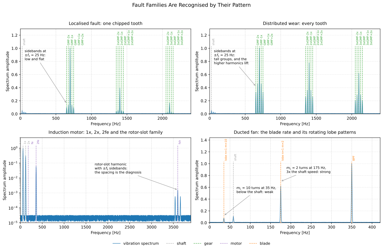
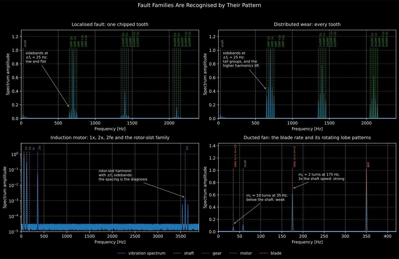
A fault family is recognised by its pattern, not by a single number. The two gear panels are the same 28-tooth pinion at 1500 r/min with two different faults: a chipped tooth gives low, flat sidebands at $\pm f_s$ and harmonics that fall away; distributed wear gives tall sideband groups and lifts the higher harmonics. The motor panel spans three decades of amplitude, which is why the rotor-slot harmonic and its $\pm f_s$ sidebands need a logarithmic axis to be visible at all beside 1x. The fan panel puts the two lobe patterns beside the blade rate they come from.

Show the code for this figure

import matplotlib.pyplot as plt
import numpy as np

# The library predicts the lines; the spectra under them are synthesised at
# exactly those frequencies, so the figure and the printed values agree.
gear = gear_mesh_frequencies(1500.0, 28, harmonics=3, sidebands=2)
freq = np.linspace(0.0, 2400.0, 4800)
amp = np.full_like(freq, 0.004)
for order, height in enumerate((1.0, 0.40, 0.16), start=1):
    for centre, level in (
        (order * gear["GMF"], height),
        (order * gear["GMF"] - gear.shaft_rate, 0.13 * height),
        (order * gear["GMF"] + gear.shaft_rate, 0.13 * height),
    ):
        amp += level * np.exp(-0.5 * ((freq - centre) / 2.2) ** 2)

spectrum = type("S", (), {"frequencies": freq, "amplitude": amp})()
gear.within(1.0, 2400.0).plot(spectrum=spectrum)
plt.show()

5. From a raw record to a named line

The kinematics answer where to look; the signal chain answers what is there. Before either, something has to record the machine, and envelope analysis is unusually sensitive to how that is done.

Step 0. Getting the record

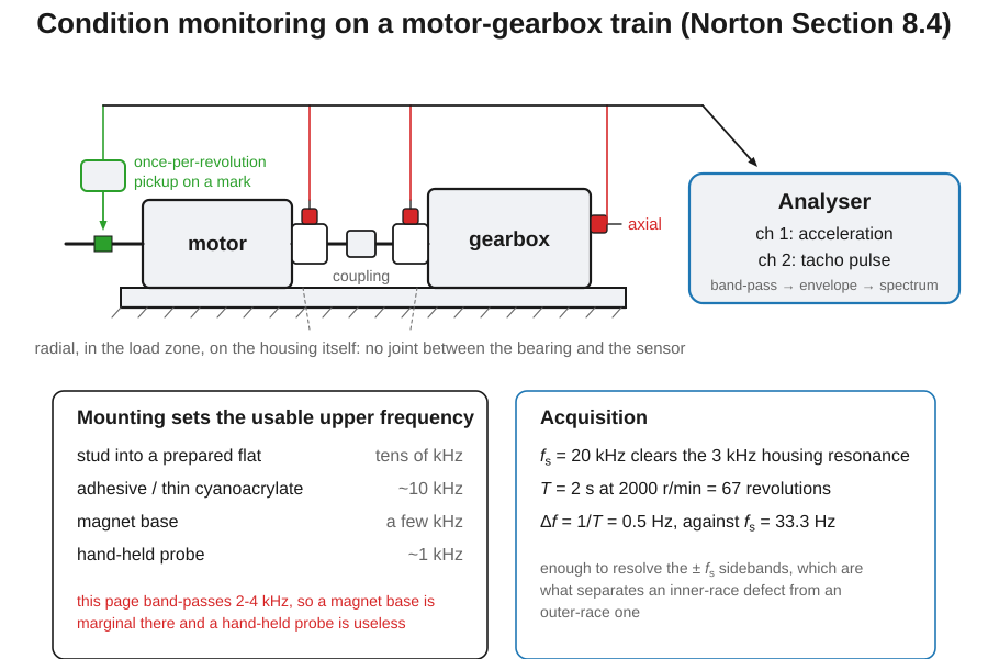
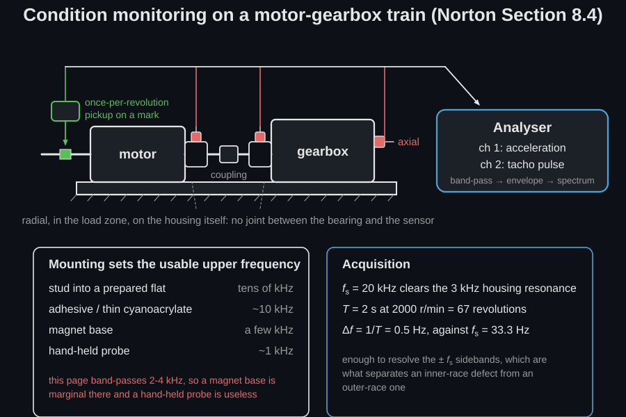
Where the transducer goes. On the bearing housing, in the load zone, as close to the outer race as the geometry allows and with the shortest possible structural path to it. A measurement taken across a bolted joint, on a guard or on sheet metal loses the high-frequency impact energy the whole method rests on. Radial and axial positions answer different questions: radial (horizontal, or vertical where the load direction demands it) for the bearing and unbalance families, axial for misalignment and for helical or bevel gear meshes.

How it is mounted. The mounting resonance sets the usable upper frequency, and this method needs kilohertz. A stud mount into a prepared flat reaches tens of kilohertz; an adhesive or thin cyanoacrylate bond a little less; a magnet base typically a few kilohertz; a hand-held probe barely one. The band used below is 2-4 kHz, which a magnet base is marginal at and a hand probe cannot reach — this is the single most common reason an envelope analysis finds nothing on a bearing that is in fact spalled.

What to acquire. The sample rate must clear the ringing resonance with margin: 20 kHz for a 3 kHz housing resonance leaves the band-pass and the detector room to work. The record must contain enough revolutions for the envelope spectrum to resolve the shaft rate, because the resolution the reader gets is $1/T$ and the sideband spacing to be resolved is $f_s$ itself. Two seconds at 2000 r/min is 67 revolutions and 0.5 Hz of resolution against a 33 Hz shaft rate, which is why the shaft line and the $\pm f_s$ sidebands of section 1 are separable at all. Record longer if the speed is low or the sidebands are the diagnosis; record shorter only if the speed will not hold still (see The speed is the whole prediction above).

Which transducer. An ordinary piezoelectric accelerometer covers the kilohertz bands used here. An acoustic-emission or dedicated high-frequency sensor moves the useful band up by an order of magnitude, which changes the band step 1 should isolate; if the machine is instrumented that way, find the resonance before choosing it.

The three signal-processing steps

For a bearing the classical route has three steps, and the library has one function for each:

1. Isolate the resonance the impacts ring. A spall excites a high-frequency structural resonance of the housing, far above the shaft harmonics and the gear mesh. Pass its band as band=(low, high) to envelope_spectrum, which band-passes the record with a zero-phase filter before the detector so the modulation phase is untouched. Choosing that band is the only judgement in the chain: look at the raw spectrum for the broadband hump the impacts excite, tap the housing and watch what rings, or scan band centre and width for the band whose envelope is most impulsive (the kurtogram). The band must sit above the shaft harmonics, the gear mesh and its sidebands and any electrical line, or those tones survive the band-pass and appear as their own lines in the envelope spectrum, where a mesh peak is easily misread as a bearing harmonic. It must be wide enough to pass the impact ringing without truncating it and narrow enough that the noise floor does not swamp it. The 2-4 kHz used on this page is chosen because these impacts ring a 3 kHz housing resonance.
2. Detect and transform the envelope. The repetition rate of the impacts is an amplitude modulation of that resonance, so it becomes a line in the envelope spectrum, at the fault frequency and its harmonics. See the cepstrum and envelope-spectrum guide.
3. Name the lines. Overlay the kinematic prediction. .plot(spectrum=…) accepts any envelope_spectrum result (or anything exposing frequencies and amplitude) and draws the predicted lines over it, coloured by family so shaft harmonics never read as bearing evidence.

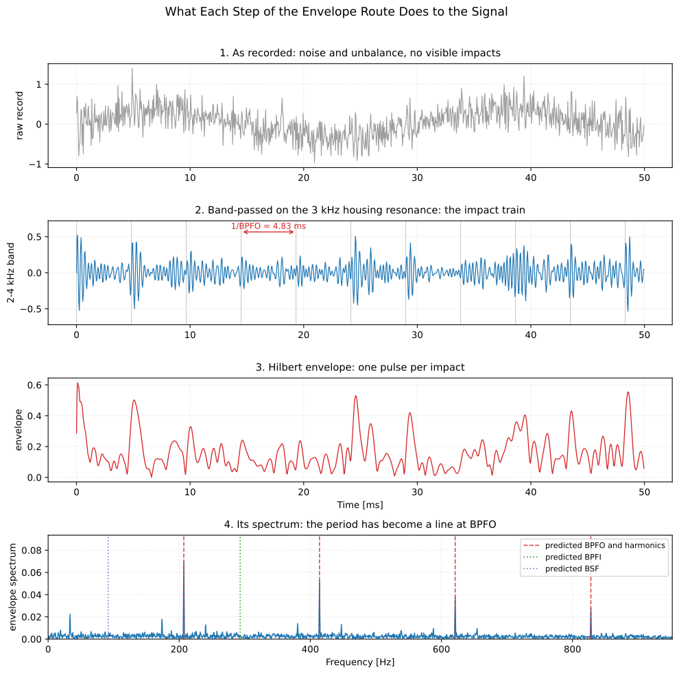
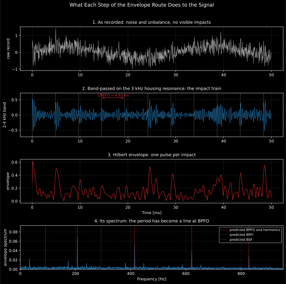
The three steps made visible on one record. The impacts are invisible in the raw signal, obvious once the 2-4 kHz band is isolated, rectified into a pulse train by the envelope detector, and finally read as a line at 207 Hz and its harmonics — the period of panel 2 becoming the frequency of panel 4.

Show the code for this figure

import matplotlib.pyplot as plt
from scipy import signal as sp_signal

# The record x, its sample rate fs, its time base t and the predicted BPFO
# are the ones built for the opening figure.
band = (2000.0, 4000.0)
spec = envelope_spectrum(x, fs, band=band)     # carries .envelope and .times

# The same zero-phase 4th-order Butterworth band-pass the call applies
# internally, run here so the intermediate record can be drawn.
sos = sp_signal.butter(4, band, btype="bandpass", fs=fs, output="sos")
narrow = sp_signal.sosfiltfilt(sos, x)

fig, axes = plt.subplots(4, 1, figsize=(10, 10))
window = slice(0, int(0.05 * fs))                       # the first 50 ms
axes[0].plot(t[window], x[window]); axes[0].set_ylabel("raw a")
axes[1].plot(t[window], narrow[window]); axes[1].set_ylabel("2-4 kHz")
axes[2].plot(spec.times[window], spec.envelope[window])
axes[2].set_ylabel("envelope"); axes[2].set_xlabel("Time [s]")
keep = spec.frequencies <= 4.6 * bpfo
axes[3].plot(spec.frequencies[keep], spec.amplitude[keep])
for order in range(1, 5):
    axes[3].axvline(order * bpfo, ls="--", color="C1")
axes[3].set_xlabel("Frequency [Hz]"); axes[3].set_ylabel("envelope spectrum")
plt.show()

Two more tools help when the record is crowded. Time synchronous averaging removes everything not locked to one shaft, which separates a gearbox’s two shafts before the sidebands are read; and the cepstrum collapses a whole harmonic or sideband family onto a single quefrency spike, which is the fastest way to tell which periodicity dominates when several are superimposed.

Put the two together on one machine. The record below is the one the figures on this page are drawn from: two seconds at 20 kHz from a stud-mounted accelerometer on the bearing housing, radial and in the load zone, with the shaft speed taken from the once-per-revolution pickup at the same moment. The bearing supports a 28-tooth pinion, so the housing carries three families at once.

from phonometry import (
    bearing_fault_frequencies,
    combine_fault_lines,
    envelope_spectrum,
    gear_mesh_frequencies,
)

record, fs = x, 20000.0          # the housing record and its sample rate
shaft_rpm = 2000.0               # from the tacho, not from the nameplate

# The bearing's own lines, the mesh family of the pinion it supports, and the
# shaft harmonics. Put them all on one axes.
bearing = bearing_fault_frequencies(shaft_rpm, 15, 6.0, 34.0,
                                    contact_angle_deg=12.96)
gear = gear_mesh_frequencies(shaft_rpm, 28, harmonics=2, sidebands=1)
lines = combine_fault_lines(bearing, gear)

spectrum = envelope_spectrum(record, fs, band=(2000.0, 4000.0))
lines.within(1.0, 1600.0).plot(spectrum=spectrum)

within(low, high) trims the family to the span the analysis actually covers, which matters because the highest mesh harmonic here (2xGMF+1x, 1900 Hz) is above the useful part of this envelope spectrum.

Covered and not covered

• Covered

  The kinematic families of Norton Section 8.4: rolling-contact bearings (Eqs. 8.4 to 8.14), gear mesh and sidebands (Eq. 8.3), induction-motor supply, slip, pole-pass and rotor-slot lines (Eqs. 8.19 and 8.20), and blade-passing frequencies with the lobed interaction patterns of a ducted axial fan (Eqs. 8.15 to 8.18), through bearing_fault_frequencies, gear_mesh_frequencies, induction_motor_frequencies, blade_pass_frequencies, combine_fault_lines and shaft_rate.

• Not covered

  These are predictions, not detections: nothing here decides whether a line is present, only where it would be. The amplitude criteria that turn a present line into a severity assessment (crest factor and kurtosis trends, ISO 10816 / ISO 20816 velocity severity bands) are outside this module; Norton’s own guidance is qualitative (crest factors of 2.5 to 3.5 for a healthy bearing, up to about 11 with impulsive defects; kurtosis near 3 healthy and above 4 damaged). The pole-pass frequency $\text{FP}=p\times f_{\text{slip}}$ is standard condition-monitoring practice rather than Norton’s: he gives the slip frequency itself as the broken-bar sideband spacing and does not multiply it by the pole count.

See also

• Cepstrum, echoes and the envelope spectrum: the envelope spectrum these lines are drawn on, and the cepstral collapse of a harmonic family.
• Time synchronous averaging: separating one shaft’s signature from everything asynchronous with it.
• Mechanical mobility and the FRF family (ISO 7626-1): finding the structural resonances a defect impact excites.
• Bending-wave transmission at plate junctions: what happens to the vibration once it leaves the machine.
• API reference: vibration.machinery.diagnostics.

References

• Norton, M. P., & Karczub, D. G. (2003). Fundamentals of noise and vibration analysis for engineers (2nd ed.). Cambridge University Press. https://doi.org/10.1017/CBO9781139163927Section 8.4 collects the discrete fault frequencies of rotating machinery implemented on this page: the eleven rolling-contact bearing frequencies after Shahan and Kamperman (Eqs. 8.4-8.14), the gear-meshing frequency (Eq. 8.3), the blade-passing frequency and the lobed interaction patterns of a ducted axial fan (Eqs. 8.15-8.17), the pump hydraulic pulsation frequency (Eq. 8.18) and the induction-motor supply and rotor-slot harmonic frequencies (Eqs. 8.19-8.20). ISBN 978-0-521-49913-2.