Cepstrum, echoes and the envelope spectrum

The spectral estimators describe what frequencies a signal contains; this page covers what hides in the shape of that spectrum. The cepstrum - the inverse Fourier transform of the log spectrum - lives in phonometry.signals and turns two hard spectral problems into easy peak-picking: periodic spectral ripple (an echo, a harmonic family) collapses onto a single spike at the quefrency of its period, and the smooth spectral envelope separates from the fine structure by plain windowing - liftering - in the quefrency domain. The same machinery extends the Hilbert envelope with an envelope spectrum in which amplitude modulations become discrete lines.

The whole trick is a chain of four steps: the logarithm turns a multiplicative echo into additive spectral ripple, and the inverse FFT collapses that ripple onto a single quefrency spike.

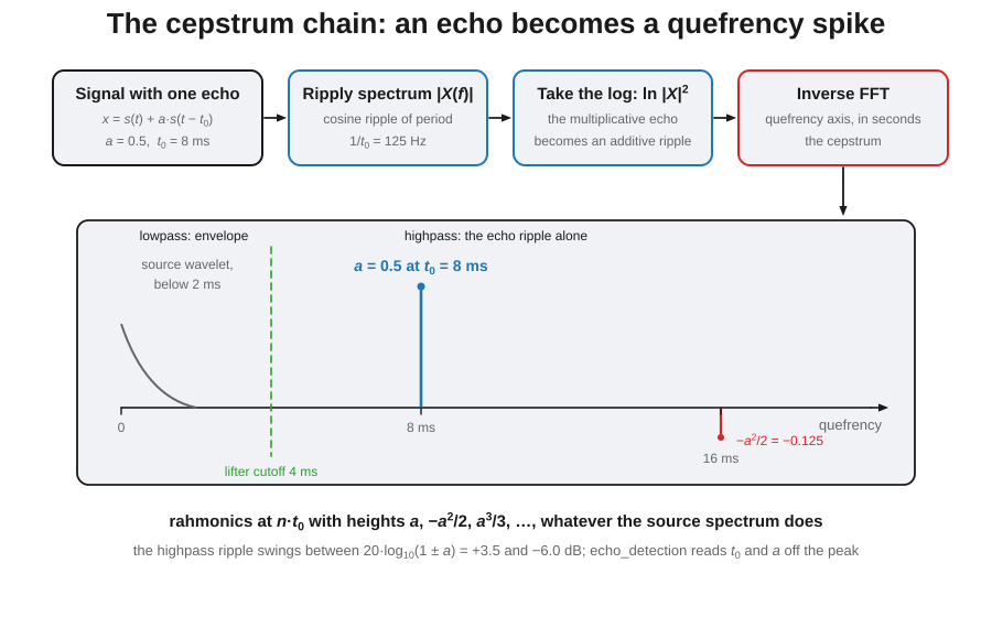
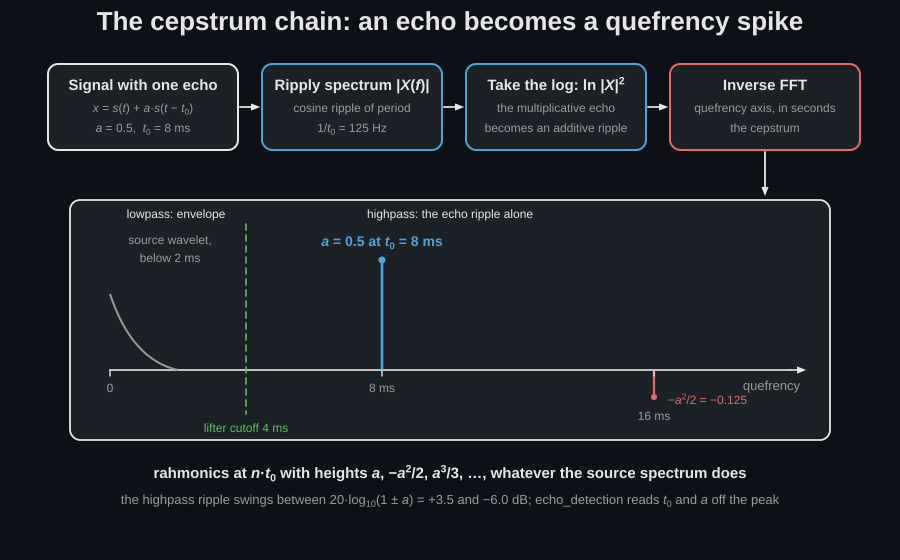
The vocabulary is Bogert’s deliberate wordplay on the domain it mirrors, which is the one fact that makes the names memorable rather than arbitrary:

Term	Mirrors	What it is	Units
cepstrum	spectrum	the spectrum of a log spectrum	signal units
quefrency	frequency	its independent variable	seconds
rahmonics	harmonics	the peaks repeating along it at $n{t}_0$	seconds
liftering	filtering	selecting a range of it	—

1. The cepstrum and its three variants

Because the log turns the convolution $x=h\ast u$ into the sum $\ln X=\ln H+\ln U$, components that overlap in the spectrum add - and separate - in the cepstral domain (Havelock Ch. 27, Eqs. (22)-(23)). cepstrum computes the three standard variants over the quefrency axis:

• 'power' (default): the inverse DFT of $\ln |X{|}^2$ (Milner’s Fig. 21). Real, even and phase-blind - the workhorse for echo and harmonic-family detection. This is Milner’s signed cepstrum of the log-power spectrum; Bogert’s original 1963 “power cepstrum” squares once more and is non-negative - the library follows Milner throughout, so negative rahmonics keep their sign;
• 'real': the inverse DFT of $\ln |X|$ - exactly half the power cepstrum, and the quantity whose causal folding is the minimum-phase reconstruction (below);
• 'complex': the inverse DFT of $\ln |X|+j\arg X$ with the phase unwrapped and its linear component removed (Havelock Ch. 87, Eq. (14)). It keeps the phase, so it is invertible: the entry point to homomorphic deconvolution.

import numpy as np
from phonometry import cepstrum

fs = 48000.0
rng = np.random.default_rng(1)
x = rng.standard_normal(4096)

res = cepstrum(x, fs, kind="power")
print(res.quefrencies[:3], res.cepstrum.shape)   # quefrency axis, in s
res.plot()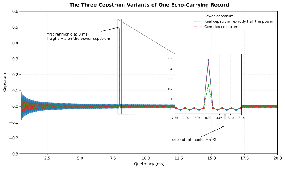

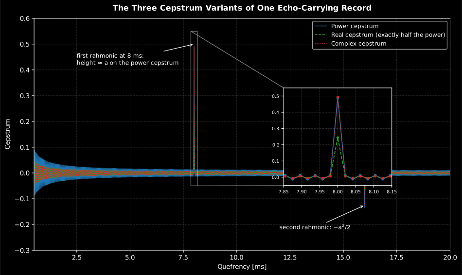
The three variants of one echo-carrying record (a band-limited wavelet plus a reflection at 8 ms, $a=0.5$). All three carry the rahmonics at 8 and 16 ms with heights $a$ and $-a^2/2$ (Milner’s signed convention); the inset shows the real cepstrum at exactly half the power cepstrum, and the source wavelet concentrates below 2 ms.

Show the code for this figure

import matplotlib.pyplot as plt
import numpy as np
from scipy import signal as sp_signal
from phonometry import cepstrum

fs = 48000.0
# A band-limited source wavelet plus one reflection at 8 ms (a = 0.5)
b, a = sp_signal.butter(2, 0.3)
s = np.zeros(4096)
s[37:37 + 256] = sp_signal.lfilter(b, a, np.r_[1.0, np.zeros(255)])
x = s + 0.5 * np.roll(s, 384)

# One line per variant — each CepstrumResult draws itself:
cepstrum(x, fs, kind="power").plot()
plt.show()

# The three variants overlaid by hand on one quefrency axis:
fig, ax = plt.subplots()
for kind, style in (("power", "-"), ("real", "--"), ("complex", ":")):
    res = cepstrum(x, fs, kind=kind)
    q_ms = 1e3 * res.quefrencies
    mask = (q_ms > 0.5) & (q_ms <= 20.0)
    ax.plot(q_ms[mask], res.cepstrum[mask], style, label=f"{kind} cepstrum")
ax.set(xlabel="Quefrency [ms]", ylabel="Cepstrum")
ax.legend()
plt.show()

The result carries the full periodic quefrency axis (0 .. (nfft-1)/fs); quefrencies above nfft/(2·fs) are the mirrored negative quefrencies, where the even power and real cepstra repeat and the complex cepstrum keeps its anticausal (non-minimum-phase) content. Zero-padding via nfft reduces cepstral time-aliasing when the log spectrum has sharp features, exactly like the oversample padding of minimum_phase.

2. Echo detection: the rahmonic spike train

A single reflection $x(t)=s(t)+as(t-t_0)$ multiplies the spectrum by $1+a{e}^{-j2\pi f{t}_0}$ - a ripple of period $1/t_0$ across the whole band. Its logarithm expands, for $|a|<1$, into the exactly summable series

$$\ln \left(1+a{e}^{-j\theta }\right)=\sum _{n\ge 1}(-1{)}^{n+1}\frac{a^n}{n}{e}^{-jn\theta },$$

so the cepstrum carries a spike train at the rahmonics $n{t}_0$ with amplitudes $a,-a^2/2,a^3/3,\dots$ (their sum is $\ln (1+a)$), regardless of the spectrum of $s$ itself, which concentrates at low quefrencies. On the signed cepstrum of the log-power spectrum (kind='power', Milner’s convention) the first spike’s height is the reflection coefficient $a$ - of either sign - plus whatever the source cepstrum contributes at that quefrency (negligible for broadband sources, whose cepstrum concentrates at low quefrencies); on an ideal impulse-plus-echo the identity is a closed form the tests and the conformance suite pin to 1e-10. echo_detection automates the reading: it picks the largest |cepstrum| peak in the searched band (so an inverting reflection, $a<0$, is found at its true delay rather than missed), refines the delay by quadratic interpolation through the peak and its neighbours, and reports the signed peak value as the reflection coefficient. When the true delay falls between samples the rahmonic splits across quefrency bins: the interpolated delay still lands on it, but the reported coefficient underestimates $|a|$ (down to about 65 % of it midway between samples).

import numpy as np
from phonometry import echo_detection

fs = 48000.0
rng = np.random.default_rng(2)
s = rng.standard_normal(12000)               # broadband source
x = s + 0.5 * np.roll(s, 384)                # echo: 8 ms, a = 0.5

res = echo_detection(x, fs, min_quefrency=0.002)
print(res.delay, res.reflection_coefficient)  # 0.008 s, ~0.5
res.plot()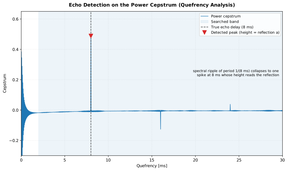

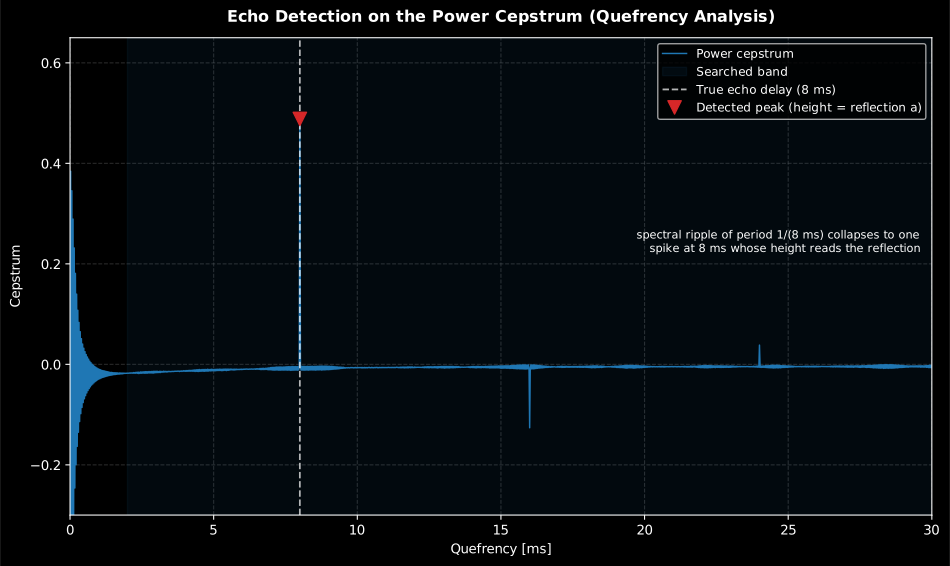
The cepstrum reads the echo off the axis rather than off the waveform: the detected peak lands at 8.000 ms and stands 0.488 high against the true $a=0.5$. The confirmation is the small negative spike at 16.0 ms, −0.126 against the series’ $-a^2/2=-0.125$: an unrelated spectral periodicity has no reason to produce an alternating rahmonic train, so the second spike is what separates an echo from a coincidence. Everything left of the shaded band is the source’s own envelope, which is why the search starts above it.

Show the code for this figure

import matplotlib.pyplot as plt
import numpy as np
from scipy import signal as sp_signal
from phonometry import echo_detection, noise_signal

fs = 48000.0
n = 12000
impulse = np.zeros(n)
impulse[0] = 1.0
b, a = sp_signal.butter(2, [0.004, 0.9], btype="bandpass")
direct = sp_signal.lfilter(b, a, impulse)              # broadband click
ir = direct + 0.5 * np.roll(direct, int(0.008 * fs))   # echo at 8 ms
ir += noise_signal(fs, n / fs, color="white", rms=1e-4, seed=13)

res = echo_detection(ir, fs, min_quefrency=0.002)

fig, ax = plt.subplots(figsize=(10, 6))
half = res.nfft // 2 + 1
ax.plot(1e3 * res.quefrencies[:half], res.cepstrum[:half], lw=1.1)
ax.axvline(8.0, ls="--", color="k", label="True echo delay")
ax.plot([1e3 * res.delay], [res.reflection_coefficient], "v", ms=10,
        label="Detected peak (height = reflection a)")
ax.set_xlim(0.0, 30.0)
ax.set_xlabel("Quefrency [ms]")
ax.set_ylabel("Cepstrum")
ax.legend()
plt.show()

The searched band starts above the low-quefrency region occupied by the source’s own spectral envelope (min_quefrency, default 16 samples) and ends at the unambiguous half of the axis (max_quefrency). The seismic reverberation spike trains of Havelock Ch. 87 are the same signature at geophysical scale. Note the negative second rahmonic at $2t_0$ in the figure: the $-a^2/2$ term of the series, a useful confirmation that a peak really is an echo and not an unrelated spectral periodicity.

From a measured impulse response

Everything above runs on a synthetic click, and the input the method actually consumes is an impulse response. Measure it with any of the library’s excitations — an exponential sweep, an MLS, or the Golay pair of system measurement — keep the direct sound and the reflection inside one record, and pass the impulse response straight to echo_detection.

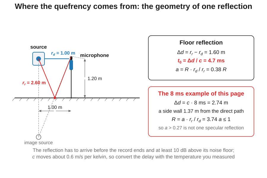
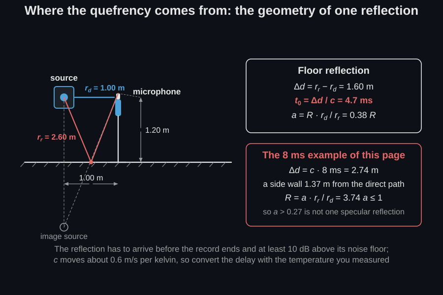
The delay is a path-length difference. $\Delta d=c{t}_0$, so the page’s 8 ms at 343 m/s means the reflected path is 2.74 m longer than the direct one, which fixes the reflector once the source and receiver positions are known. Convert with the temperature you measured, not with 343: the speed of sound moves by about 0.6 m/s per kelvin, which is 0.2 % on the distance for every degree.

The coefficient is an amplitude ratio at the microphone, not a surface property. $a=0.5$ means the reflection arrives at half the amplitude of the direct sound — a quarter of the energy — and the two together ripple the magnitude spectrum between $+3.5$ and $-6.0$ dB, which is the ripple section 3 isolates. But $a$ already contains the extra spherical spreading of the longer path, so the surface’s own reflection factor is $R=a(r_{\text{reflected}}/r_{\text{direct}})$. For an 8 ms delay over a 1 m direct path that ratio is 3.74, so $R=3.74a$ — a number that cannot exceed one, which means an apparent $a$ above $1/(1+c{t}_0/r_{\text{direct}})$ is not a single specular reflection at all. Where $R$ is valid, the absorption coefficient at that angle of incidence is $\alpha =1-R^2$; the absorption pages own the standardized routes to the same quantity.

A negative peak is a phase inversion. A pressure-release boundary — or an inverted electrical path — flips the sign of the reflection, and the whole rahmonic series flips with it.

Four conditions decide whether the number means anything:

1. min_quefrency above the duration of the direct arrival, so the source’s own spectral envelope is outside the search band.
2. The reflection at least 10 dB above the noise floor of the response.
3. The second rahmonic present at $2t_0$ with the opposite sign — the check that separates a real echo from an unrelated spectral periodicity.
4. An analysed span several times the delay being sought. The ripple has period $1/t_0$ in frequency and a record of length $T$ resolves the spectrum only to $1/T$; gating the response around the arrivals of interest also keeps later reflections from adding rahmonics of their own.

3. Liftering: envelope versus fine structure

Filtering in the quefrency domain is called liftering (Havelock Ch. 27, Sec. 4.3). A lowpass lifter keeps the quefrencies below the cutoff and returns the smooth log-spectral envelope with the ripple removed; a highpass lifter keeps the complement - the ripple alone. The two modes are exactly complementary in dB, because the split is linear in the log domain:

import numpy as np
from phonometry import lifter

fs = 48000.0
rng = np.random.default_rng(3)
s = rng.standard_normal(12000)
x = s + 0.5 * np.roll(s, 384)                # the same 8 ms echo

low = lifter(x, fs, cutoff=0.004, mode="lowpass")    # envelope of ln|X|
high = lifter(x, fs, cutoff=0.004, mode="highpass")  # the echo ripple
print(np.allclose(low.liftered_db + high.liftered_db, low.spectrum_db))
low.plot()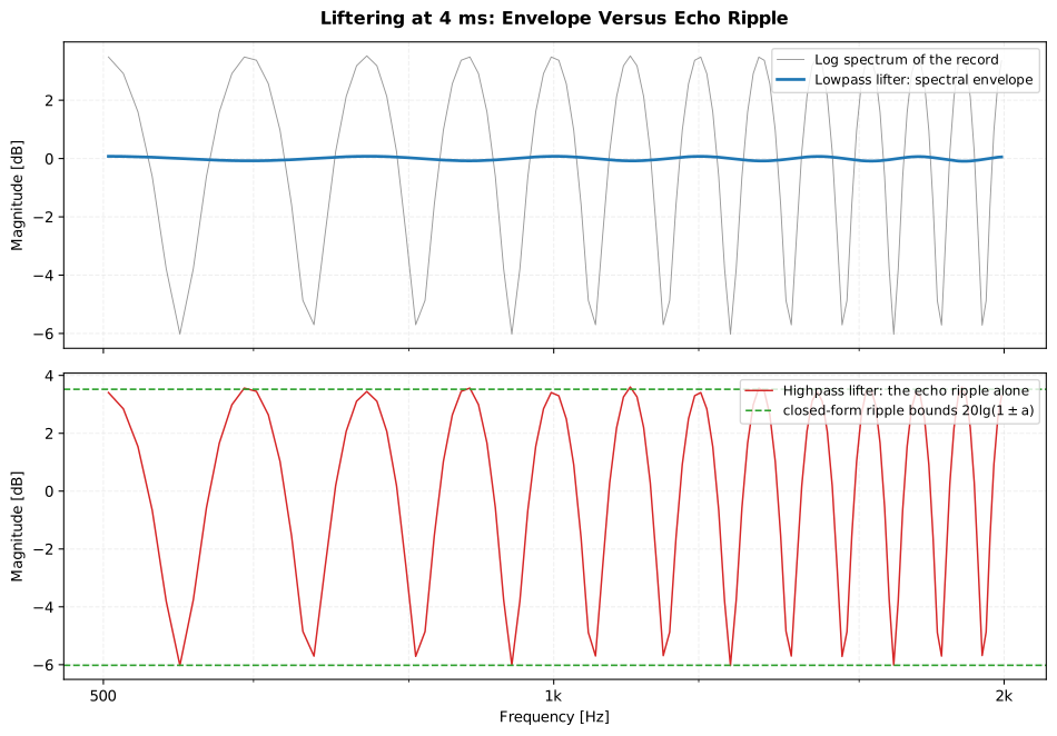

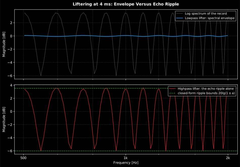
The 4 ms lifter split on a pure-echo record: the lowpass side returns the smooth spectral envelope, the highpass side isolates the echo’s 125 Hz ripple, swinging exactly between the closed forms $20{\log }_{10}(1\pm a)=+3.5$ and $-6.0$ dB.

Show the code for this figure

import matplotlib.pyplot as plt
import numpy as np
from scipy import signal as sp_signal
from phonometry import lifter

fs = 48000.0
# A band-limited wavelet carrying a pure 8 ms echo (a = 0.5), so the
# highpass ripple has the exact closed-form bounds.
b, a = sp_signal.butter(2, 0.3)
s = np.zeros(4096)
s[37:37 + 256] = sp_signal.lfilter(b, a, np.r_[1.0, np.zeros(255)])
x = s + 0.5 * np.roll(s, 384)

low = lifter(x, fs, cutoff=0.004, mode="lowpass")
high = lifter(x, fs, cutoff=0.004, mode="highpass")

# One line — the cepstrum with the cutoff and the two log spectra:
low.plot()
plt.show()

# The envelope/ripple split by hand, zoomed on 500-2000 Hz:
band = (low.frequencies >= 500) & (low.frequencies <= 2000)
fig, axes = plt.subplots(2, 1, sharex=True)
axes[0].semilogx(low.frequencies[band], low.spectrum_db[band], "0.6",
                 lw=0.7, label="Log spectrum")
axes[0].semilogx(low.frequencies[band], low.liftered_db[band], lw=2,
                 label="Lowpass lifter: envelope")
axes[1].semilogx(high.frequencies[band], high.liftered_db[band], "r",
                 label="Highpass lifter: ripple")
for bound in (20 * np.log10(1.5), 20 * np.log10(0.5)):
    axes[1].axhline(bound, color="g", linestyle="--")
axes[1].set_xlabel("Frequency [Hz]")
for ax in axes:
    ax.set_ylabel("Magnitude [dB]")
    ax.legend()
plt.show()

For the pure-echo signal the highpass ripple swings between the closed forms $20{\log }_{10}(1+a)$ and $20{\log }_{10}(1-a)$ dB, another oracle the tests pin. In speech analysis the identical operation separates the vocal-tract envelope (formants) from the excitation harmonics; here it is the general tool for “smooth versus periodic” splits of any measured magnitude response.

4. The complex cepstrum and the minimum-phase connection

The complex cepstrum keeps the unwrapped phase, so the transform is a round trip: CepstrumResult.invert() restores the record to machine precision, including the linear-phase (pure delay) component that the forward transform removes and stores in linear_phase_samples:

import numpy as np
from scipy import signal as sp_signal
from phonometry import cepstrum

fs = 48000.0
x = np.zeros(2048)
b, a = sp_signal.butter(2, 0.3)
x[37:293] = sp_signal.lfilter(b, a, np.r_[1.0, np.zeros(255)])

res = cepstrum(x, fs, kind="complex")
print(res.linear_phase_samples)              # negative: a bulk delay removed
print(np.max(np.abs(res.invert() - x)))      # ~1e-14
res.plot()   # the complex cepstrum against quefrency (as in the figure above)

Between the log and the inverse transform anything can be edited - that is homomorphic deconvolution (Havelock Ch. 87, Sec. 3.3): zero the rahmonics to remove an echo, keep only the low quefrencies to extract a source wavelet. A minimum-phase signal has a causal complex cepstrum, which is why folding the real cepstrum onto positive quefrencies reconstructs the minimum phase from $|H|$ alone: minimum_phase and phase_decomposition run on that same folding core (Bendat & Piersol Sec. 13.1.4; Tohyama in Havelock Ch. 75 edits reverberation by manipulating exactly these causal/anticausal parts).

The round trip above is exact to machine precision because the record is smooth, noiseless and close to minimum phase. The complex cepstrum is not robust in general, and the reason is the phase. It needs an unwrapped phase that can be followed continuously across the whole band, and wherever the magnitude approaches zero — a deep null, a zero near the unit circle — the phase turns by $\pi$ in the space of a bin or two and the unwrapper can jump the wrong way. Every quefrency downstream then inherits the error. The power and real cepstra are immune, because they never look at phase at all.

Three guards. Zero-pad with nfft so the phase is sampled finely enough for the unwrapper to track it; keep the record’s signal-to-noise ratio high in the bands that matter, since additive noise randomises the phase exactly where the magnitude is small; and check the round trip with invert() before trusting any edited cepstrum — a failed unwrap shows up immediately as a reconstruction error far above 1e-10. When the record cannot support it, use the power cepstrum for detection and the real-cepstrum folding of minimum_phase when only a magnitude-consistent phase is needed.

5. The envelope spectrum: modulations as lines

Where the cepstrum finds periodicities of the spectrum, the envelope spectrum finds periodicities of the amplitude. Bendat & Piersol Section 13.3 (Fig. 13.11) formalizes the structure: an envelope detector, a DC remover, and a spectral view of what remains. envelope_spectrum runs the Hilbert envelope (kind="magnitude", the practical default) or the book’s square-law detector (kind="squared") through exactly that chain, scaled by the taper’s coherent gain so a sinusoidal modulation whose frequency falls on an analysis bin reads out as a line at its exact amplitude (off-bin lines read low by the taper’s scalloping loss, up to about 1.4 dB for the default Hann). The optional band=(low, high) argument reproduces the band-pass front end of the book’s Fig. 13.11 - the classical bearing-envelope chain: isolate the structural-resonance band excited by the defect impacts with a zero-phase band-pass, then envelope it - so an out-of-band interferer is strongly attenuated before the detector (the roll-off of a fourth-order Butterworth applied forward and backward; the rejection is finite, and the zero-phase pass leaves small transients at the record edges).

For an AM tone $A_0(1+m\cos (2\pi f_{m}t))\cos (2\pi f_{c}t)$ with $f_m$ on an analysis bin the closed forms are:

kind	mean level	line at $f_m$	line at $2f_m$
'magnitude'	$A_0$	$A_{0}m$	-
'squared'	$A_0^2(1+m^2/2)$	$2A_0^{2}m$	$A_0^2{m}^2/2$

import numpy as np
from phonometry import envelope_spectrum

fs = 8192.0
t = np.arange(int(4 * fs)) / fs
x = (1.0 + 0.4 * np.cos(2 * np.pi * 25.0 * t)) * np.cos(2 * np.pi * 1000.0 * t)

res = envelope_spectrum(x, fs)
k = int(round(25.0 * res.nfft / fs))
print(res.mean_level, res.amplitude[k])      # ~1.0 and ~0.4
res.plot()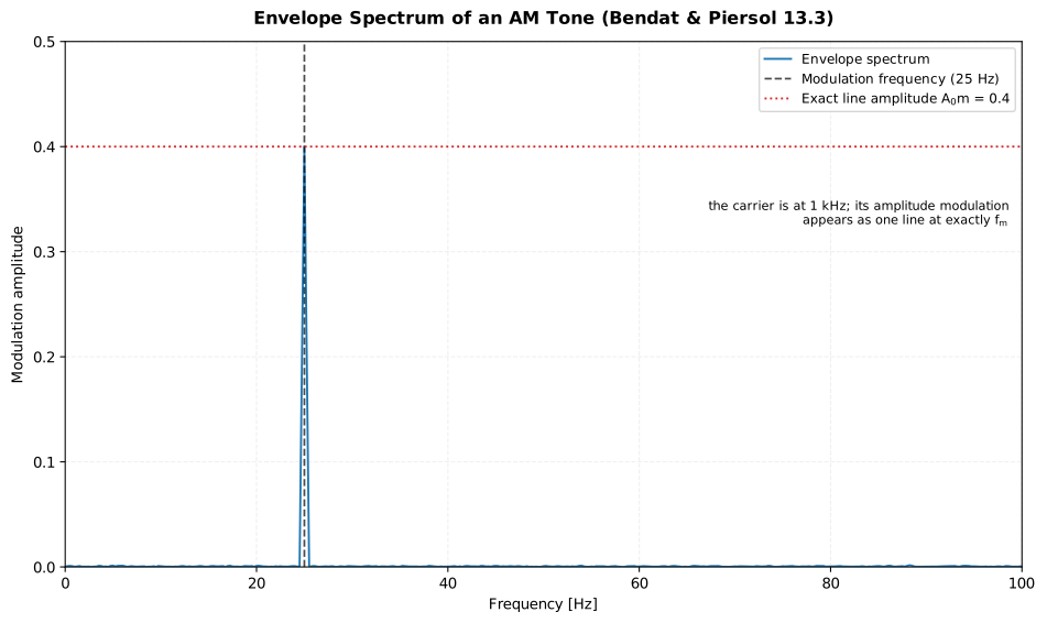

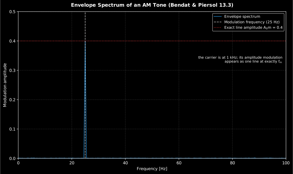
The line is not proportional to the modulation, it is the modulation: with $f_m$ on an analysis bin the magnitude detector reads 0.3996 against the closed form $A_{0}m=0.4$, and mean_level reads 1.001 against $A_0=1$. That is the point of the scaling by the taper’s coherent gain — the ordinate is a modulation depth, not an arbitrary level. Around it the floor sits near 5×10⁻⁴, so the line stands about 58 dB clear even with white noise at 3 % of the carrier, which is why the chain finds bearing defects that the carrier’s own spectrum hides.

Show the code for this figure

import matplotlib.pyplot as plt
import numpy as np
from phonometry import envelope_spectrum, noise_signal

fs = 8192.0
seconds = 4.0
t = np.arange(int(seconds * fs)) / fs
x = (1.0 + 0.4 * np.cos(2 * np.pi * 25.0 * t)) * np.cos(2 * np.pi * 1000.0 * t)
x += noise_signal(fs, seconds, color="white", rms=0.03, seed=8)

res = envelope_spectrum(x, fs)

fig, ax = plt.subplots(figsize=(10, 6))
ax.plot(res.frequencies, res.amplitude, lw=1.4, label="Envelope spectrum")
ax.axvline(25.0, ls="--", color="k", label="Modulation frequency")
ax.axhline(0.4, ls=":", color="r", label=r"Exact line amplitude $A_0 m$")
ax.set_xlim(0.0, 100.0)
ax.set_xlabel("Frequency [Hz]")
ax.set_ylabel("Modulation amplitude")
ax.legend()
plt.show()

Bearing and gear defects, mains hum and wind-turbine amplitude modulation all appear this way: lines at the modulation frequency and its harmonics, cleanly separated from the carrier’s own spectrum. The envelope mean removed by the DC step is kept in mean_level (the carrier amplitude for the magnitude detector), and remove_dc=False skips the remover when the absolute DC line matters.

Choosing the band, and mounting the sensor

The band argument is where the bearing chain is won or lost, and neither the band nor the transducer is a free choice.

The band. Run a plain spectrum of the raw record first and look for the broad hump the defect impacts excite — a structural resonance of the housing, typically somewhere between 1 and 20 kHz for rolling-element bearings. Put the band around that hump. Make it several times wider than the highest repetition rate you need to see (three to five times the highest defect frequency, so its harmonics survive the detector), and choose $f_s$ at least 2.56 times the top of the band. Where two candidate humps exist, take the one whose envelope spectrum gives the higher line-to-floor ratio: the band is a signal-to-noise choice, not a physical constant. A band too wide readmits the strong low-frequency components the front end exists to remove; one too narrow starves the envelope of impact energy; and the zero-phase pass leaves transients at both record edges, so trim them before reading amplitudes.

The mounting. The usable upper frequency is set by the mounted resonance of the accelerometer, not by the sensor’s own datasheet limit, and that is exactly the band the bearing chain needs. Stud mounting or a thin layer of adhesive keeps a general-purpose accelerometer usable to roughly 10 kHz; a magnet base typically collapses that to a couple of kilohertz and a hand-held probe to about 1 kHz — that is, the mounting alone can destroy the band the method depends on. Put the sensor on the bearing housing, in the load zone, as close to the outer race as the machine allows, with its axis in the load direction and the cable strain-relieved. ISO 5348 is the mounting reference.

# A 3 kHz structural resonance rung at a 120 Hz defect rate, under a 50 Hz
# line three times as strong: the band-pass is what separates them.
t_s = np.arange(int(4 * fs)) / fs
ring = np.sin(2 * np.pi * 3000.0 * t_s) * np.exp(-(t_s % (1 / 120.0)) / 0.001)
raw = ring + 3.0 * np.sin(2 * np.pi * 50.0 * t_s)

wide = envelope_spectrum(raw, fs)
narrow = envelope_spectrum(raw, fs, band=(2000.0, 4000.0))
k120 = int(round(120.0 * wide.nfft / fs))
print(round(wide.amplitude[k120], 4),        # 0.0093 — buried
      round(narrow.amplitude[k120], 4))      # 0.1964 — 26 dB better

The lines the chain produces are identified by frequency, not by amplitude, and the kinematic families that name them — ball-pass outer and inner race, ball spin, cage, gear mesh and its shaft-rate sidebands — are computed from the geometry and the shaft speed at Machine fault frequencies, which draws them straight onto an envelope spectrum like this one. Running the envelope on the residual of a synchronous average first removes the deterministic gear components and leaves the bearing lines clear.

Relation to the other estimators

The cepstrum starts from the same one-record FFT conventions as the calibrated spectral estimators, and its folding core is literally the one inside minimum_phase - the refactor is pinned bit-exact in the tests. The envelope spectrum is the frequency-domain view of the same analytic signal the Hilbert envelope returns in time, and a natural pre-analysis before the dedicated wind-turbine amplitude-modulation metrics: the envelope spectrum tells you whether and at what rate a signal is modulated, the domain metrics quantify it normatively.

What this guide covers

• Covered

  The three cepstrum variants and liftering of Havelock, Kuwano and Vorländer’s Handbook of Signal Processing in Acoustics (cepstrum, lifter, Chapters 27 and 87), the single-echo delay and reflection coefficient read off the power cepstrum (echo_detection), the invertible complex cepstrum and its homomorphic round trip (CepstrumResult.invert), and the Bendat & Piersol Chapter 13 envelope spectrum (envelope_spectrum) with its closed-form AM tone lines.

• Not covered

  echo_detection picks only the single largest cepstral peak in the searched band, so a response with several overlapping echoes needs manual peak-picking or repeated calls on narrowed bands; it is not a multi-echo separator. The module also has no mel-warped or MFCC-style cepstrum for perceptual audio features: lifter and cepstrum work on the plain linear-frequency log spectrum only.

See also

• Correlation, time delay and envelope: the Hilbert envelope this page transforms into a spectrum.
• Calibrated spectral analysis: the log spectrum the cepstrum starts from.
• Time synchronous averaging: removing the synchronous part before running an envelope spectrum on the residual.
• Machine fault frequencies: the bearing and gear families read off exactly this envelope spectrum.
• Swept-sine distortion: the minimum-phase folding that shares this page’s core.
• API reference: signals.cepstrum.

References

• Bendat, J. S., & Piersol, A. G. (2010). Random data: Analysis and measurement procedures (4th ed.). Wiley. https://doi.org/10.1002/9781118032428Section 13.1.4 (the Hilbert relation between log magnitude and phase behind the minimum-phase folding) and Section 13.3 with Figure 13.11 (envelope detection followed by DC removal, the structure of the envelope spectrum). ISBN 978-0-470-24877-5.
• Havelock, D., Kuwano, S., & Vorländer, M. (Eds.). (2008). Handbook of signal processing in acoustics. Springer. https://doi.org/10.1007/978-0-387-30441-0Chapter 27 (Milner: the cepstral transform as the inverse DFT of the log power spectrum, quefrency, lowpass/highpass liftering), Chapter 87 (Neelamani: the complex cepstrum, homomorphic deconvolution, periodic spike trains from reverberation) and Chapter 75 (Tohyama: minimum-phase/all-pass manipulation in the cepstral domain). ISBN 978-0-387-77698-9.
• International Organization for Standardization. (2021). Mechanical vibration and shock — Mechanical mounting of accelerometers (ISO 5348:2021). The mounting methods behind the usable upper frequency of an envelope-analysis measurement: stud and adhesive mounting against magnet bases and hand-held probes.