A sound level meter is calibrated for sound arriving from one direction, its reference direction, and most of the sound it measures arrives from all of them: the reverberant field of a room, the traffic of a street, the machinery of a workshop. Its microphone and its case are not transparent at high frequency, so a meter that reads a plane wave from the front correctly reads a field from every direction low. IEC 61183:1994 gives the two ways of finding by how much. The free-field method rotates the instrument in an anechoic room and weights the reading for each direction by the share of the sphere it stands for; the diffuse-field method compares the instrument with a reference instrument in a reverberation room.
This page runs both on a synthetic meter: a microphone whose pattern has, at each frequency, the directivity Table B.1 of the standard prints for a type LS2aP/LS2F laboratory standard microphone, mounted on a case that narrows it in the plane the case sits in.
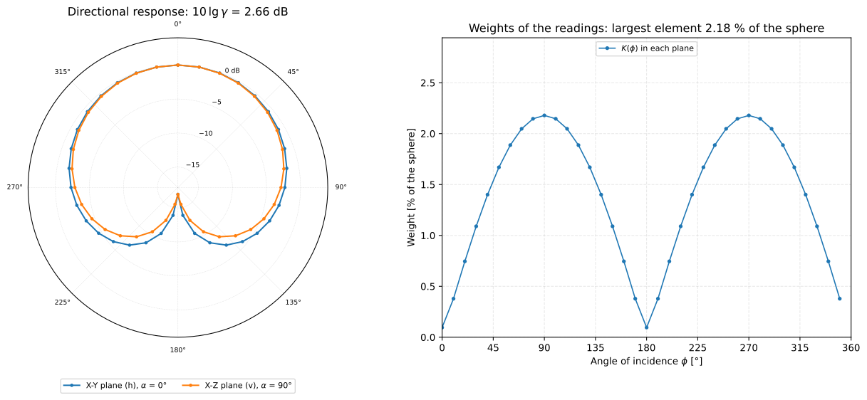
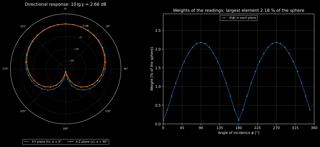
The response of the meter at 8 kHz in the two planes of Annex A (left), and
the weight each reading takes in the sum (right), from the result’s own
.plot().
1. The directivity factor
Section titled “1. The directivity factor”What the standard needs is the ratio of what the meter reads for a plane wave from its reference direction to what it reads, on average over the sphere, for the same wave from every direction. That ratio is the directivity factor of Formula (2), written in Formula (3) with the angle from the reference direction and the angle of the plane about it:
An omnidirectional meter has ; one that favours its reference direction has . The random-incidence sensitivity level is then the free-field sensitivity level for the reference direction less the directivity index (Formula (1)):
depends on the individual meter, only on its dimensions and geometry, so one measurement of serves every meter of a model (4.2).
How the measurement goes
Section titled “How the measurement goes”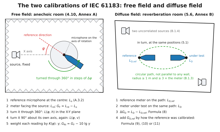
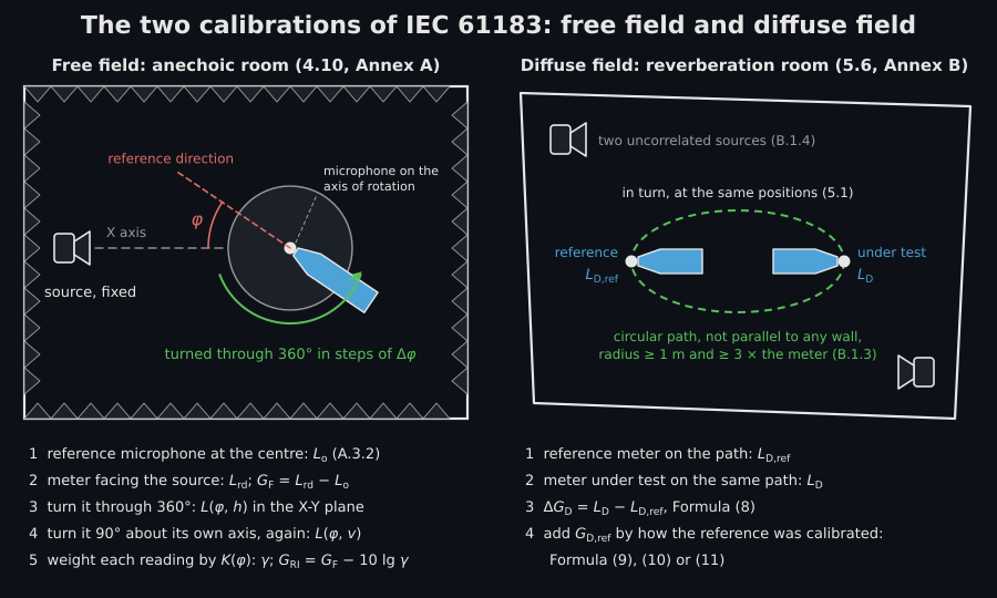
The meter is turned in front of a fixed source in an anechoic room (left), or compared with a reference on the same path in a reverberation room (right). The library takes over once the levels are read.
| Requirement | Value | Clause |
|---|---|---|
| Anechoic room | Meets ISO 3745; pure tones or random noise, bands no wider than one-third octave, filters of IEC 61260 class 0 or 1 | 4.10 |
| Source | Far enough that the level varies by less than ±1 dB within 0,3 m of the microphone | A.2.2 |
| Signal | At least 20 dB above the background, and held constant during each rotation | A.2.3 |
| Turntable | The acoustical centre of the microphone on the axis of rotation, the reference direction and the source in the plane of rotation | A.2.1, A.4.2 |
| Rotations | 360° in the X-Y plane, then the meter turned 90° about its own axis and 360° again, the X-Z plane | A.4.5, A.4.6 |
| Angular step | Small enough that no element of the sphere exceeds 3 %; 10° leaves 2,2 % | A.1.6, A.1.7 |
| Pure tones | and may need the rms average of at least eight tones per one-third-octave band, spaced evenly on a logarithmic axis | 4.11 |
| Reverberation room | Meets ISO 3741; broadband or filtered random noise, bands no wider than one-third octave | 5.6 |
| Integration time | Long enough that repeated results scatter by less than 0,05 dB: 2 min from 500 Hz, 8 min from 250 Hz, 15 min from 125 Hz, longer below | 5.6, B.1.4 |
| Microphone path | Both microphones moved in turn along the same circular path, not parallel to any wall, of radius the larger of 1 m and three times the largest dimension of the meter; two uncorrelated omnidirectional sources of about equal power help the diffusivity | B.1.3, B.1.4 |
| Reference meter | A directivity factor as near unity as possible; a type LS2aP/LS2F or LS2bP microphone is recommended | B.1.1, B.1.2 |
2. Readings in two planes, and what each is worth
Section titled “2. Readings in two planes, and what each is worth”In practice the integral becomes a sum over a limited number of directions, each reading taken to stand for the element of the sphere around it (Formula (4)). Annex A rotates the meter through 360° in the X-Y plane, turns it 90° about its axis, and rotates it again, which is the X-Z plane: two planes, the angle in equal steps . The elements are rings cut into quarters by the planes, so a reading at 90° stands for far more of the sphere than one near the axis, and Formulas (A.1) and (A.2) give the factor each reading is weighted with:
from phonometry import metrology
k = metrology.adjustment_factors(10.0)   # 36 factors, 0° to 350°print(k[[0, 1, 9]].round(5))             # [0.00095 0.00378 0.02179]print(round(2 * k.sum(), 12))            # 1.0print(round(100 * metrology.largest_element_fraction(10.0), 2))  # 2.18
Those are the first, second and last rows of Table A.1, and all ten of its rows
come out to the five decimals it prints. A.1.6 asks for the largest element to
be no more than 3 % of the sphere; at 10° steps it is the one at 90°, 2,18 %,
the “approximately 2,2 %” of A.1.7. A step of 15° would leave 3,26 %, and
adjustment_factors then warns with a SphereDivisionWarning. Any step that
divides 180° works, and planes=4 gives the four planes at 45° that NOTE 2 of
A.6 asks for when the reference direction is not normal to the diaphragm: every
factor halves.
The 72 factors sum to one only when the readings at 0° and 180° enter both sums of Formula (A.3), and the paragraph under it could be read otherwise: it says those readings are the same in the two planes and “have only to be taken into account once”. They have to be measured once. Each plane’s pole factor covers half the polar cap, so counted in one sum only, the factors add up to 0,998 097: the sum loses times the energy read at each pole, and comes out high by . That is 0,008 dB for a meter that reads the same in every direction, and it grows with the directivity: about 0,02 dB at dB. The library counts the poles in both sums, and the omnidirectional meter has exactly.
The directivity factor is Formula (A.3), one row of readings per plane:
import numpy as np
def pattern_db(phi_deg, n, floor=0.02):    """L(phi) - L_rd of a meter whose squared pressure is (1 - b)[(1 + cos phi)/2]^n + b."""    lobe = ((1 + np.cos(np.radians(phi_deg))) / 2) ** n    return 10 * np.log10((1 - floor) * lobe + floor)
phi = np.arange(0, 360, 10)levels = 94.0 + np.vstack((pattern_db(phi, 0.785),    # X-Y plane (h), 8 kHz                           pattern_db(phi, 0.98)))    # X-Z plane (v), the case narrows itd = metrology.directivity_factor(levels)print(round(d.gamma, 3), round(d.directivity_index_db, 2))   # 1.845 2.66d.plot()                  # the polar response, one curve per planed.plot(view="weights")    # K(phi) of each reading
The reference level defaults to the reading at 0° in the first
plane, which A.4.4 takes with the meter in that very position; pass
reference_level_db= when it was measured separately.
3. One plane, or 38 equal elements
Section titled “3. One plane, or 38 equal elements”A meter that is rotationally symmetric about its reference direction needs one rotation only (NOTE 1 of A.4.7), and Formula (A.4) counts that plane twice:
a = metrology.axisymmetric_directivity_factor(levels[0])print(round(a.directivity_index_db, 2)) # 2.45That is the X-Y plane alone, whose pattern was built to have the 2,45 dB Table B.1 prints for the microphone at 8 kHz; the case of the synthetic meter is what adds the other 0,21 dB in the two-plane result.
The note to A.1.8 offers the other way round: place the directions so that the elements are equal, 38 of them at 2,6 % of the sphere each, and every reading weighs the same (Formula (A.5)). Each direction here halves its element’s area in polar angle, which reproduces the list the note prints:
horizontal, vertical = metrology.equal_area_incidence_angles()print(horizontal[:6].round(1)) # [ 0. 32.6 50.8 65.1 77.8 90. ]e = metrology.equal_area_directivity_factor( 94.0 + pattern_db(horizontal, 0.785), 94.0 + pattern_db(vertical, 0.98))print(round(e.directivity_index_db, 2)) # 2.66The note prints 77,9° and 282,1° where the construction gives 77,85° and 282,15°. All the other pairs of the printed list sum to 180,0° about the grazing direction, and 77,9° + 102,2° is 180,1°: the two are in the errata register. A tenth of a degree does not move a directivity factor, but the list is not symmetric as printed.
4. The random-incidence sensitivity level, band by band
Section titled “4. The random-incidence sensitivity level, band by band”With measured at each band and from the free-field calibration of A.3 ( with the meter in place, with a free-field reference microphone in its stead), Formula (1) gives the random-incidence sensitivity level. Here the synthetic meter is measured at every preferred frequency Table B.1 prints, its X-Y plane given the of the microphone at that band, and its free-field sensitivity level rolls off above 10 kHz:
bands = sorted(metrology.IEC61183_TABLE_B1)   # the 30 preferred frequencies, 25 Hz to 20 kHz
def meter(frequency_hz):    """The synthetic meter at one band: the X-Y plane has the 10 lg gamma Table B.1    prints for the microphone, and the case narrows the X-Z plane."""    target = metrology.IEC61183_TABLE_B1[frequency_hz].directivity_index_db    n = 0.98 / (10 ** (-target / 10) - 0.02) - 1   # the exponent with that index    return metrology.directivity_factor(        94.0 + np.vstack((pattern_db(phi, n), pattern_db(phi, 1.25 * n))))
index = [meter(f).directivity_index_db for f in bands]g_f = -10 * np.log10(1 + (np.array(bands) / 25000) ** 4)   # L_rd - L_o at each bandr = metrology.random_incidence_sensitivity(bands, g_f, index)shown = np.isin(r.frequencies_hz, [1000, 4000, 8000, 16000])print(r.correction_db[shown].round(2))              # [-0.06 -0.95 -2.66 -5.62]print(r.random_incidence_level_db[shown].round(2))  # [-0.06 -0.95 -2.71 -6.29]r.plot()                      # G_F and G_RIr.plot(view="correction")     # G_RI - G_F = -10 lg gamma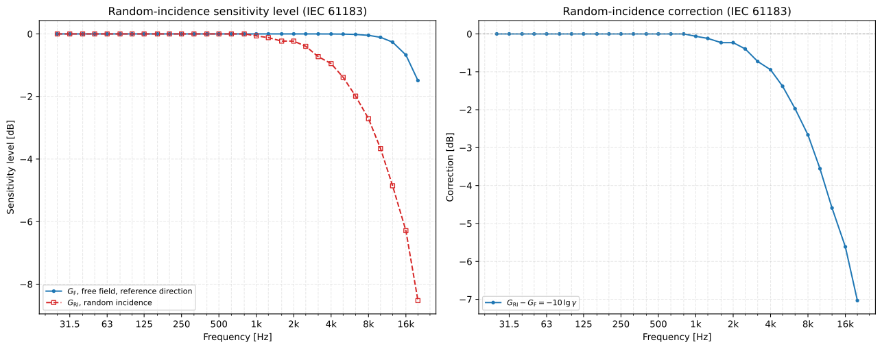
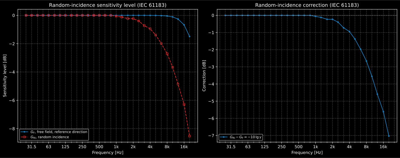
and of the synthetic meter at every preferred frequency Table B.1 prints (left), and the correction between them (right).
The correction is what a meter calibrated in a free field reads low in a random-incidence field: negligible up to about 1 kHz, where the wavelength is large against the microphone, and several decibels by 10 kHz. It is why a meter is specified for one field or the other. IEC 61672-1:2013 applies its frequency-weighting limits to the free-field response or to the random-incidence response, as applicable (5.5.4), and has the random-incidence response determined by the free-field method of IEC 61183 (5.5.5), the method of this page. A meter flat for a plane wave from the front reads a random-incidence field low by this correction, and one flat in a random-incidence field reads that plane wave high by it: it cannot be flat for both.
5. The diffuse-field method
Section titled “5. The diffuse-field method”The second method needs no anechoic room. The meter under test and a reference meter are placed in turn at the same positions in a reverberation room, and the difference of what they indicate (Formula (8)) is added to the diffuse-field sensitivity level of the reference, known in one of three ways:
Annex B recommends a type LS2aP/LS2F or LS2bP laboratory standard
microphone as the reference, and Table B.1 prints, for the first, both its and from 25 Hz to 20 kHz.
metrology.IEC61183_TABLE_B1 holds the table, and Formulas (10) and (11) take
their correction from it unless told otherwise:
In an 80 dB diffuse field each instrument indicates the field plus its own diffuse-field sensitivity level: the meter its random-incidence level (1.2), and a reference LS2aP whose pressure sensitivity level is 0 dB its :
print(metrology.IEC61183_TABLE_B1[8000.0])# ReferenceMicrophoneRow(directivity_index_db=2.45, diffuse_pressure_difference_db=1.2)
delta_dp = np.array([metrology.IEC61183_TABLE_B1[f].diffuse_pressure_difference_db                     for f in bands])dd = metrology.diffuse_field_sensitivity(    bands,    80.0 + r.random_incidence_level_db,  # L_D, the meter under test    80.0 + delta_dp,                     # L_D,ref, a pressure-calibrated LS2aP    reference_pressure_level_db=0.0,     # G_P,ref; Delta_DP from Table B.1)print(dd.reference_correction_db[shown])            # [0.   0.25 1.2  3.05]print(dd.diffuse_field_level_db[shown].round(2))    # [-0.06 -0.95 -2.71 -6.29]dd.plot()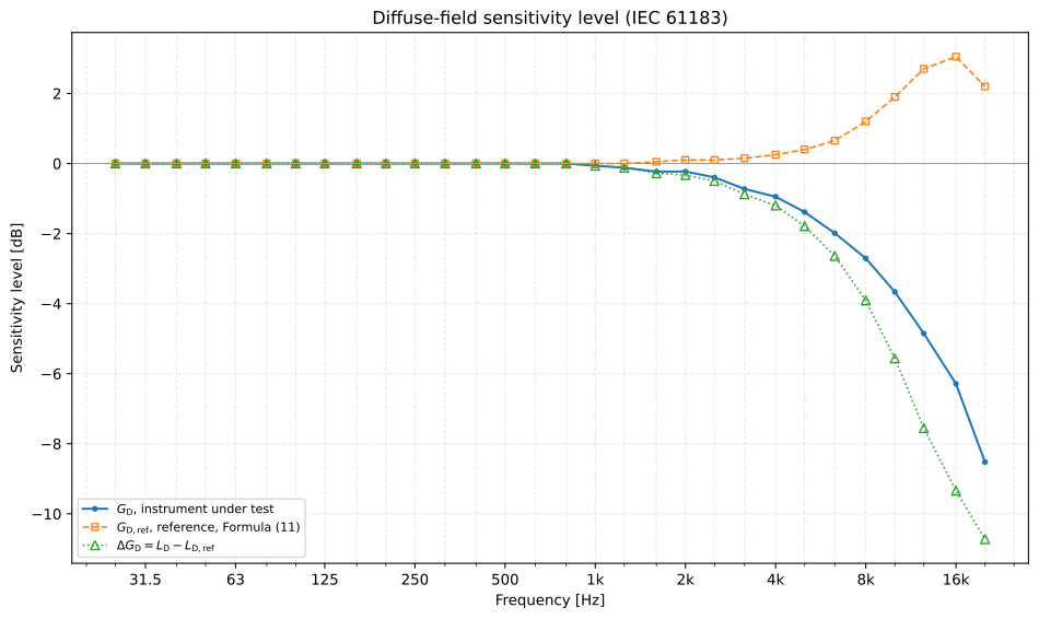
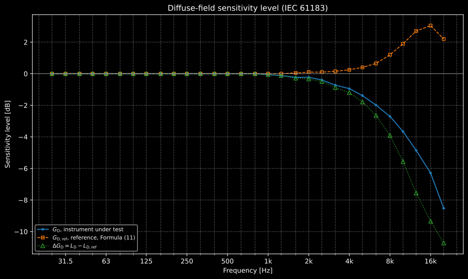
Formula (11) on the synthetic meter: the pressure-calibrated reference reads the diffuse field high by , and adding it back to the level difference returns the meter’s own diffuse-field level, which is its random-incidence level (1.2).
The two methods meet here: for the purpose of the standard the diffuse-field
sensitivity level may be used interchangeably with the random-incidence one
(1.2), and the example returns, from a comparison in a room, the level the
first method measured in an anechoic room. reference_free_field_level_db
selects Formula (10) and reference_random_incidence_level_db Formula (9);
reference_directivity_index_db and
reference_diffuse_pressure_difference_db replace the Table B.1 defaults for a
reference microphone of another type.
Show the code for these figures
import matplotlib.pyplot as plt
fig = plt.figure(figsize=(13.5, 6.0))d.plot(fig.add_subplot(1, 2, 1, projection="polar"))d.plot(fig.add_subplot(1, 2, 2), view="weights")fig.tight_layout()
fig, (ax_levels, ax_correction) = plt.subplots(1, 2, figsize=(13.5, 5.4))r.plot(ax_levels)r.plot(ax_correction, view="correction")fig.tight_layout()
fig, ax = plt.subplots(figsize=(10, 6))dd.plot(ax)fig.tight_layout()plt.show()
What this guide covers
Section titled “What this guide covers”Covered
IEC 61183:1994, the calculations of both methods: the adjustment factors of Formulas (6), (7), (A.1) and (A.2) for any angular step that divides the half circle and any number of planes, with the halving of NOTE 2 of A.6 and the doubling of Formula (A.4); the largest element of the division and the 3 % criterion of A.1.6, as a warning; the directivity factor from two or more planes (Formula (A.3)), from one plane under rotational symmetry (Formula (A.4)) and from 38 equal-area elements (Formula (A.5)), with the directions of the note to A.1.8; the random-incidence sensitivity level of Formulas (1) and (A.6); the diffuse-field sensitivity level by the three routes of Formulas (8) to (11); and Table B.1, which supplies the reference corrections. Table A.1 is reproduced to its five decimals, and the 2,2 % of A.1.7 and the 2,6 % of the note to A.1.8 are reproduced.
Not covered
The measurements themselves: the anechoic room of ISO 3745 and the reverberation room of ISO 3741 the standard requires, the placement of the source and of the meter on its turntable, the signal-to-noise ratio of A.2.3 and the integration times of B.1.4. The averaging of at least eight tones within a one-third-octave band of 4.11 is left to the caller, who passes the averaged level of each band. The corrections of IEC 62585 that bring a measurement made with a sound calibrator, a comparison coupler or an electrostatic actuator to the meter’s free-field response are on their own page; its corrections for the case, the microphone and the windscreen (clauses 9 to 11) are not implemented.
References
Section titled “References”- International Electrotechnical Commission. (1992). Measurement microphones — Part 1: Specifications for laboratory standard microphones (IEC 61094-1:1992). The type LS2aP/LS2F and LS2bP laboratory standard microphones Annex B recommends for the reference instrument of the diffuse-field method, whose characteristics Table B.1 prints.
- International Electrotechnical Commission. (1994). Electroacoustics — Random-incidence and diffuse-field calibration of sound level meters (IEC 61183:1994). The implemented method: the directivity factor of Formulas (2) to (5) and (A.3) to (A.5), the adjustment factors of Formulas (6), (7), (A.1) and (A.2) and their halving in NOTE 2 of A.6, the 3 % criterion of A.1.6, the random-incidence sensitivity level of Formulas (1) and (A.6), the diffuse-field sensitivity level of Formulas (8) to (11), and Table B.1. Read from BS EN 61183:1995, the English text of EN 61183:1994, which is IEC 1183:1994 unchanged.