Time Weighting

A displayed sound level is always a time-weighted level: before anything reaches the readout, the squared, frequency-weighted pressure passes through an exponential detector whose time constant sets how quickly the level follows the signal. This page is that detector, implemented as a sample-exact recursive filter: the Fast and Slow characteristics of IEC 61672-1:2013 (clause 5.8), the legacy asymmetric Impulse ballistics, streaming state for block processing, and the toneburst verification against the standard’s Table 4.

The names are older than the mathematics. FAST and SLOW were literal descriptions of a needle movement, standardized for analog meters in ANSI S1.4-1983 and IEC 60651 and carried into IEC 61672-1 as the F and S exponential constants; IMPULSE was added in the same era for impact noise and has since been dropped from the requirements, surviving in instruments only for legacy procedures (the choosing guidance below says when each is defensible; Bies, Hansen & Howard 2017, §3.6 covers the instrument practice).

Two sibling pages complete the chain. The detector output is the level track that the percentile levels $L_N$ of Integrated and Statistical Levels are defined on, while the integrated metrics ($L_{eq}$, SEL) bypass the detector entirely; and the full IEC 61672-1 instrument chain that wraps this detector (weighting, ranges, periodic tests) is the subject of Build a sound level meter.

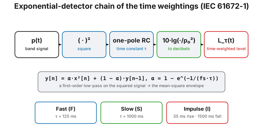
1. The exponential detector

A sound level meter’s needle cannot follow the pressure waveform: it shows a running mean square with an exponential memory. Formally (IEC 61672-1, 3.8):

$$\tau \frac{dy}{dt}+y=x^2(t)⟺y(t)=\frac{1}{\tau }{\int }_{-\infty }^t{x}^2(\xi )e^{-(t-\xi )/\tau }d\xi$$

a first-order low-pass on the squared signal. The time constant $\tau$ sets the trade-off: Fast (125 ms) follows speech-like fluctuations, Slow (1 s) steadies the readout for quasi-stationary noise. After a step onset the envelope reaches 63 % of its final value in one $\tau$ and ~99.97 % after $8\tau$; that is why level analyses discard the first instants of a recording.

2. The three time weightings

• Fast (fast): $\tau =125\text{ms}$. Standard for noise fluctuations.
• Slow (slow): $\tau =1000\text{ms}$. Standard for steady noise.
• Impulse (impulse): Asymmetric ballistics, 35 ms attack and 1.5 s decay. Both numbers are specified, not tuned: ANSI S1.4-1983 clause 2.7 defines the impulse sound level as 35 ms exponential time averaging for increasing portions of the signal and a 1500 ms time constant for decreasing portions.

A tone burst drives the RC exponential detector: the capacitor charges and drains while the Fast, Slow and Impulse meter needles follow their own ballistics, and the three level traces build up below to show the fast attack, the slow average and the asymmetric impulse hold.

Download the animation (WebM)

A tone burst drives the RC exponential detector: the capacitor charges and drains while the Fast, Slow and Impulse meter needles follow their own ballistics, and the three level traces build up below to show the fast attack, the slow average and the asymmetric impulse hold.

Download the animation (WebM)

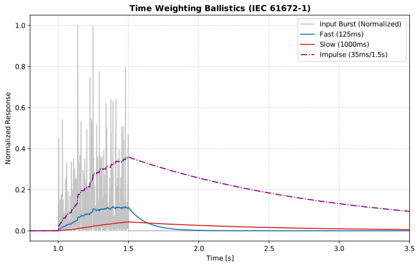
The three detectors on one 0.5 s noise burst: Fast rises and falls with it, Slow never reaches its level, and Impulse rises with Fast and then holds.

Show the code for this figure

import numpy as np
import matplotlib.pyplot as plt
from phonometry import filters

fs = 48000
t = np.arange(int(fs * 4)) / fs
burst = np.zeros_like(t)  # 0.5 s noise burst (Pa) starting at t = 1 s
rng = np.random.default_rng(42)
burst[fs:int(1.5 * fs)] = 0.2 * rng.standard_normal(int(0.5 * fs))

p0 = 2e-5
plt.figure()
for mode in ('fast', 'slow', 'impulse'):
    envelope = filters.time_weighting(burst, fs, mode=mode)
    plt.plot(t, 10 * np.log10(np.maximum(envelope, 1e-12) / p0**2), label=mode)
plt.xlabel('Time [s]')
plt.ylabel('Level [dB SPL]')
plt.legend()
plt.show()

import numpy as np
from phonometry import filters

# recording: a calibrated microphone capture (Pa) — recorded through your measurement chain. Synthesized here so the guide runs standalone.
fs = 48000
recording = 0.2 * np.sin(2 * np.pi * 1000 * np.arange(fs) / fs)

# Calculate energy envelope (Mean Square)
energy_envelope = filters.time_weighting(recording, fs, mode='fast')
# dB SPL relative to 20 μPa
spl_t = 10 * np.log10(energy_envelope / (2e-5)**2)

print(f"Steady-state Fast level: {spl_t[-1]:.1f} dB SPL")
# Steady-state Fast level: 77.0 dB SPL

The asymmetric Impulse ballistics use two constants, a fast attack and a slow decay, switching per sample on the sign of the change:

$$y[n]=y[n-1]+\alpha (x^2[n]-y[n-1]),\alpha =\{\begin{array}{ll}1-e^{-1/(f_s\cdot 0.035)}& x^2[n]>y[n-1]\\ 1-e^{-1/(f_s\cdot 1.5)}& \text{otherwise}\end{array}$$

A time constant and a decay rate are the same statement. An exponentially decaying mean square falls at a constant $10/(\tau \ln 10)$ decibels per second, which is why IEC 61672-1 clause 5.8.1 can specify F and S twice over — as design-goal constants of 0.125 s and 1 s, and as design-goal decay rates of 34.7 dB/s and 4.3 dB/s. The same arithmetic turns the 1.5 s decreasing-portion constant of the analog IMPULSE characteristic into 2.9 dB/s, the fall an operator was meant to be able to read off a moving needle.

The asymmetry has a consequence worth stating: unlike F and S, Impulse is not a filter. Its coefficient depends on the signal, so an I-weighted level is not additive — the I-weighted level of two sources running together cannot be derived from the two measured separately, while their $L_{eq}$ values can.

Choosing F, S or I

• Fast is the default of nearly every modern method: percentile levels, impulsive-event detection, community noise, the general “level vs time” plot. Its 125 ms constant is of the same order as the ear’s own loudness integration time, so an $L_{AF}$ trace roughly tracks what a listener notices.
• Slow suits quasi-stationary sources and any procedure that needs a steady readout: it averages away the flicker of a fluctuating source at the price of missing short events (a 100 ms burst peaks 7.6 dB lower on S than on F). Some legacy methods prescribe it outright, most famously aircraft-certification levels, which are built from Slow-weighted samples.
• Impulse is legacy, and deprecated for rating. It was a 1960s attempt to make a meter needle track the perceived loudness of impacts; it does not (the 35 ms attack still misses very short impulses, and the 1.5 s decay exaggerates duration). It entered the international standards with IEC 60651 and was dropped from the requirements of its successor IEC 61672-1, whose first edition (2002) explains why: I-weighted levels are not suitable for rating impulsive sounds. Modern international practice rates impulsiveness with $L_{Aeq}$ plus an adjustment (ISO 1996-1 Table A.1, or the onset analysis of Impulsive-sound prominence) and assesses hearing-damage risk with $L_{Cpeak}$, never with I-weighted levels. Some national rules still require the I weighting explicitly: the Spanish RD 1367/2007 grades its impulsive correction $K_i$ on $L_{AIeq}-L_{Aeq}$ (see Spanish Noise Regulation), which is why mode='impulse' is a first-class option here and not a compatibility shim.

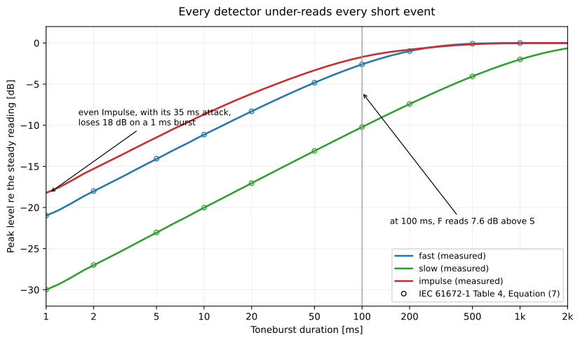
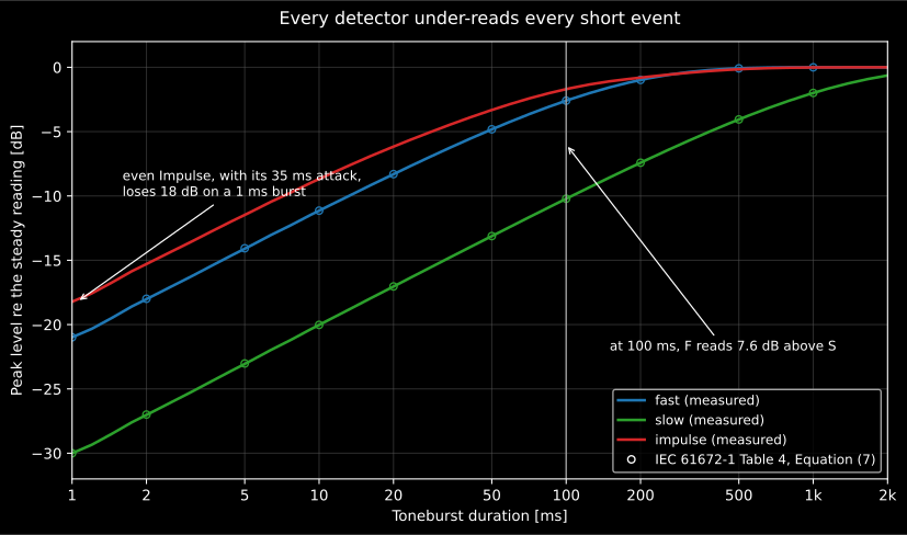
How much of an event each detector keeps, as a function of how long the event lasts. The measured curves land on the Table 4 reference points, so the whole table is one line of algebra. The gap between two curves at a given duration is the reason a maximum level has to name its time weighting; and the absolute loss is why very short impulses are rated with $L_{Cpeak}$ instead — even Impulse, the ballistics designed for impacts, is 18 dB low on a 1 ms burst.

Show the code for this figure

import numpy as np
import matplotlib.pyplot as plt

fs = 48000
t = np.arange(int(3.0 * fs)) / fs
tone = np.sin(2 * np.pi * 4000 * t)
durations = np.geomspace(0.001, 2.0, 30)

plt.figure()
for mode in ('fast', 'slow', 'impulse'):
    reference = filters.time_weighting(tone, fs, mode=mode)[int(2.5 * fs):].mean()
    peaks = []
    for t_b in durations:
        burst = np.zeros_like(t)
        stop = int(0.5 * fs) + int(t_b * fs)
        burst[int(0.5 * fs):stop] = tone[int(0.5 * fs):stop]
        peaks.append(10 * np.log10(
            filters.time_weighting(burst, fs, mode=mode).max() / reference))
    plt.semilogx(durations * 1e3, peaks, label=mode)
plt.axvline(100.0, linewidth=0.8)
plt.xlabel('Toneburst duration [ms]')
plt.ylabel('Peak level re the steady reading [dB]')
plt.legend()
plt.show()

3. time_weighting() / TimeWeighting parameters

Parameter	Type	Units	Range / default	Notes
x	1D or 2D array	pressure (any scale)	non-empty	Squared internally; output is a mean-square envelope
fs	int	Hz	> 0
mode	str	—	'fast' (default), 'slow', 'impulse'	$\tau$ = 125 ms / 1 s / 35 ms attack + 1.5 s decay
initial_state	None / 'zero' / 'first' / float / array	mean square of $x$	default None (= 'zero')	Integrator state $y[-1]$; see sections 5 and 6
TimeWeighting(fs, mode) (class)	—	—	—	Stateful variant for streaming: process(x) carries the integrator state between blocks
TimeWeighting.reset()	—	—	—	Drops the carried state so the next process() starts from rest

The output has the units of $x^2$: take 10*log10(y / p0**2) for SPL or use the level functions, which do it for you.

4. Verified ballistics (IEC 61672-1 Table 4)

Those reference values are not a lookup table with no formula behind it. IEC 61672-1 gives them in Note 1 to Table 4 as Equation (7), the exact response of the section 1 detector to an isolated 4 kHz toneburst of duration $T_b$:

$${\Delta }_{\mathrm{ref}}=10{\log }_{10}\left(1-e^{-T_b/\tau }\right)\text{dB}$$

Read it out loud and the whole table follows. On Fast ($\tau =125$ ms) a 200 ms burst gives $-0.98$ dB, a 50 ms burst $-4.82$ dB and a 10 ms burst $-11.14$ dB — the three panels below. A 100 ms burst gives $-2.59$ dB on Fast and $-10.21$ dB on Slow, and that 7.6 dB is the number quoted in the choosing guidance above. The physics is one sentence: a detector with memory $\tau$ cannot reach its steady value on an event shorter than $\tau$, so every meter under-reads every short event, by an amount that depends only on $T_b/\tau$. That is why a maximum level is meaningless without its ballistics, and why impulses short compared with 125 ms are rated with $L_{Cpeak}$ instead.

The Fast envelope’s response to 4 kHz tonebursts lands exactly on the standard’s reference values: the example below verifies the three Table 4 rows drawn in the figure; the CI suite covers the full table, from 1 s down to 1 ms for F and 1 s down to 2 ms for S, at class 1 acceptance limits:

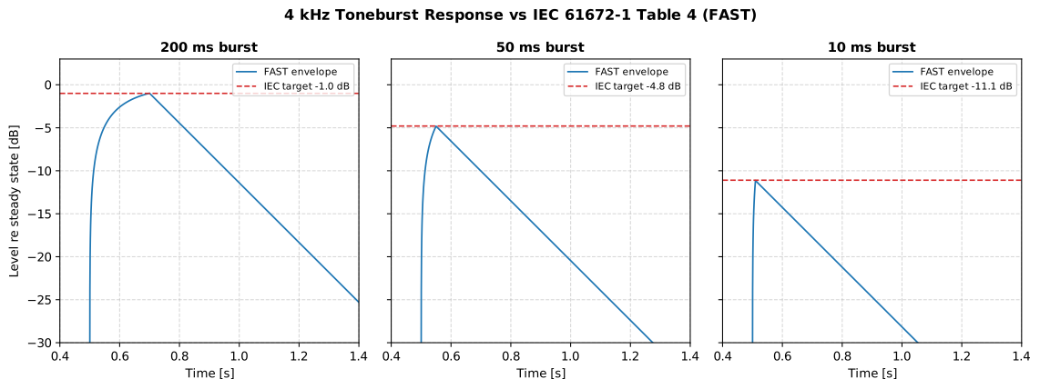
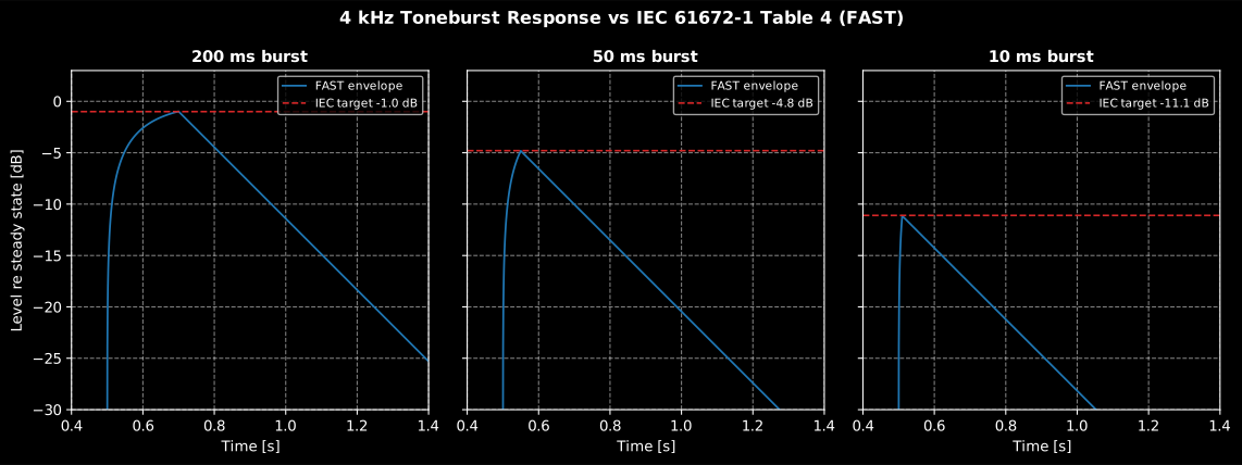
Fast envelope peaks at −1.0, −4.8 and −11.1 dB relative to the steady tone for the 200, 50 and 10 ms bursts of Table 4; the CI suite checks the full table from 1 s down to 1 ms.

Show the code for this figure

import numpy as np
import matplotlib.pyplot as plt
from phonometry import filters

fs = 48000
t = np.arange(int(fs * 2)) / fs
tone = np.sin(2 * np.pi * 4000 * t)

# Steady-state Fast reference of the continuous tone
reference = filters.time_weighting(tone, fs, mode='fast')[int(1.5 * fs):].mean()

# The three Table 4 rows the published figure draws, with their targets
cases = [(0.200, -1.0), (0.050, -4.8), (0.010, -11.1)]
fig, axes = plt.subplots(len(cases), 1, sharey=True, figsize=(8, 8))
for ax, (t_b, target) in zip(axes, cases):
    burst = np.zeros_like(t)
    stop = int(0.5 * fs) + int(t_b * fs)
    burst[int(0.5 * fs):stop] = tone[int(0.5 * fs):stop]
    envelope = filters.time_weighting(burst, fs, mode='fast')
    env_db = 10 * np.log10(np.maximum(envelope / reference, 1e-6))
    ax.plot(t, env_db, label=f'Fast envelope, {t_b * 1e3:.0f} ms burst')
    ax.axhline(target, linestyle='--', label=f'IEC target {target} dB')
    ax.set_ylabel('Level re steady state [dB]')
    ax.legend(loc='upper right')
axes[-1].set_xlabel('Time [s]')
plt.show()

5. Initial state

The integrator needs a starting value for $y[-1]$, and there are four ways to give it.

• None (the default) and 'zero' are the same thing, a start from rest, so the level climbs through the settling ramp of section 1.
• 'first' seeds it with the square of the very first sample, $x[0{]}^2$. That is an unbiased but extremely noisy estimate of the mean square — one degree of freedom — and for a tone it depends entirely on the phase at the cut. In the snippet below it is exactly zero, because a sine starting at $t=0$ starts at a zero crossing, so 'first' there is bit-identical to 'zero'.
• A float resumes a state you saved yourself, which is what block processing does in section 6.
• An array broadcastable to the input shape without the time axis does the same per channel.

If the record is a continuation of a signal already running, seed the integrator with something robust — the mean square of the first half second, initial_state=float(np.mean(recording[:fs // 2] ** 2)), is a far better estimate than a single sample. If the record is the start of the event, do not seed at all: let it start from rest and discard the first $5\tau$ (0.6 s Fast, 5 s Slow), which is exactly what ln_levels does internally before computing percentiles.

import numpy as np
from phonometry import filters

# recording: a calibrated microphone capture (Pa) — recorded through your measurement chain. Synthesized here so the guide runs standalone.
fs = 48000
recording = 0.2 * np.sin(2 * np.pi * 1000 * np.arange(fs) / fs)

# Robust seed: the mean square of the first half second, not one sample.
energy_envelope = filters.time_weighting(
    recording, fs, mode='fast',
    initial_state=float(np.mean(recording[:fs // 2] ** 2)))

6. Block processing

For block processing, pass the last output value from the previous block as the next block’s initial_state instead of resetting each block:

from phonometry import filters

state = None

# audio_blocks: consecutive frames of your calibrated recording (Pa),
#   streamed from your sound card or read from a WAV in blocks.
for block in audio_blocks:
    energy_envelope = filters.time_weighting(block, fs, mode='fast', initial_state=state)
    state = energy_envelope[-1]

For multichannel blocks with time on the last axis, carry one state per channel: use state = energy_envelope[..., -1]. A scalar initial_state is applied to every channel, while an array must match or broadcast to the non-time shape, such as (n_channels,) for input shaped (n_channels, n_samples).

Or let the TimeWeighting class carry the state for you:

from phonometry import filters

tw = filters.TimeWeighting(fs, mode='fast')
# audio_blocks: consecutive frames of your calibrated recording (Pa),
#   streamed from your sound card or read from a WAV in blocks.
for block in audio_blocks:
    energy_envelope = tw.process(block)

Concatenated block outputs are exactly equal to a single continuous call (verified for all three modes, mono and multichannel). Call tw.reset() to start from rest again.

7. Performance note

The impulse mode uses an asymmetric kernel that is JIT-compiled when numba is installed (pip install phonometry[perf]). Without numba a pure-Python fallback produces identical results, just slower.

See Integrated and Statistical Levels for $L_{eq}$/$L_N$ metrics built on these envelopes, and Why phonometry for the IEC 61672-1 tone-burst verification.

What this guide covers

• Covered

  IEC 61672-1:2013’s exponential time-weighting detector (clause 3.8) with the Fast and Slow time constants (clause 5.8.1), implemented as the recursive filter of time_weighting and the streaming TimeWeighting class, verified in CI against the class 1 tone-burst references of Table 4. The legacy asymmetric Impulse ballistics (35 ms attack, 1.5 s decay), carried into the international standards from the FAST/SLOW/IMPULSE characteristics of ANSI S1.4-1983.

• Not covered

  IEC 61672-1’s wider instrument chain (frequency weighting, level ranges, periodic tests) is not on this page; it is the subject of Build a sound level meter. ANSI S1.4-1983 is cited only for the historical origin of the F and S constants, not implemented as its own instrument specification. Modern impulsiveness rating ($L_{Aeq}$ plus an adjustment, or onset analysis) is on the Impulsive-sound prominence page, not built on the Impulse weighting here.

See also

• Levels: the percentile levels defined on the detector’s output, and the integrated metrics that bypass it.
• Build a sound level meter: the complete IEC 61672-1 instrument chain around this detector.
• Frequency Weighting: the A/C/Z filters applied before the detector.
• Block Processing: streaming the detector over frames without state discontinuities.
• Impulsive-sound prominence: the onset-based rating of impulses that the international standards moved to.
• Spanish Noise Regulation: a rating in force that still requires the I weighting, through the $L_{AIeq}-L_{Aeq}$ impulsive correction $K_i$.
• Calibration and dBFS: the IEC 61672-3 periodic tests, in which these ballistics are spot-checked against the class limits on a real instrument.
• API reference: filters.weighting.
• Theory: Time Integration: the first-order equation the exponential detectors solve, and what integrating it over a fixed block instead would change.

References

• American National Standards Institute. (1983). Specification for sound level meters (ANSI S1.4-1983). The classic analog meter specification: the FAST/SLOW dynamic characteristics the F and S constants descend from, and the IMPULSE characteristic that IEC 61672-1 no longer specifies, defined in clause 2.7 as a 35 ms exponential-time-averaging constant for increasing portions of the signal and a 1500 ms constant for decreasing portions.
• Bies, D. A., Hansen, C. H., & Howard, C. Q. (2017). Engineering noise control (5th ed.). CRC Press. https://doi.org/10.1201/9781351228152Sections 3.2 and 3.6 (sound level meters and the measurement of time-varying sound: what the F/S/I readouts mean in instrument practice). ISBN 978-1-4987-2405-0.
• International Electrotechnical Commission. (2013). Electroacoustics — Sound level meters — Part 1: Specifications (IEC 61672-1:2013). The exponential time-weighting detector (clause 3.8) with the F and S design-goal time constants and decay rates (clause 5.8.1), the maximum time-weighted sound level (clause 3.7) and its hold feature (clause 5.1.14), and the 4 kHz toneburst reference responses of Table 4 and its Equation (7) (class 1 acceptance limits) the ballistics are verified against in CI.