Correlation, time delay and envelope

Where the calibrated spectral estimators describe a signal in frequency, this page covers their time-domain counterparts in phonometry.signals: auto- and cross-correlation estimates with the three standard normalizations and their Bendat & Piersol random errors; time-delay estimation (TDE) by the direct correlator, the cross-spectrum phase slope and the generalized cross-correlation (GCC) of Knapp & Carter with the Roth, SCOT, PHAT and maximum-likelihood weightings; sub-sample peak location for impulse-response delays and alignment; and the Hilbert envelope with instantaneous phase and frequency. The GCC estimators run on the same Welch core as the spectral densities, so both views of a signal pair are mutually consistent bin by bin.

1. Correlation estimates

correlation computes the auto- or cross-correlation via zero-padded FFT so the circular product never wraps (Bendat & Piersol Section 11.4.2), with the sign convention of the book’s time-delay model: for $y(t)=\alpha x(t-{\tau }_0)+n(t)$ the estimate peaks at $\tau =+{\tau }_0$ (Eq. 5.21). Three normalizations are available:

• 'biased': the lag sums divided by $N$; tapers toward the record ends and stays bounded by $[R_{xx}(0)R_{yy}(0){]}^{1/2}$;
• 'unbiased': divided by $N-|r|$ (Eq. 11.96), an unbiased estimate of $R_{xy}(\tau )$ whose variance grows toward the ends;
• 'coefficient': the correlation coefficient function ${\rho }_{xy}(\tau )=C_{xy}(\tau )/({\sigma }_x{\sigma }_y)$ in $[-1,1]$ over the mean-removed records (Eq. 5.16).

import numpy as np
from phonometry import correlation

res = correlation(x, y, fs, normalization="coefficient", max_lag=0.05)
peak = np.argmax(res.values)
print(res.lags[peak], res.values[peak])   # delay and its coefficient
res.plot()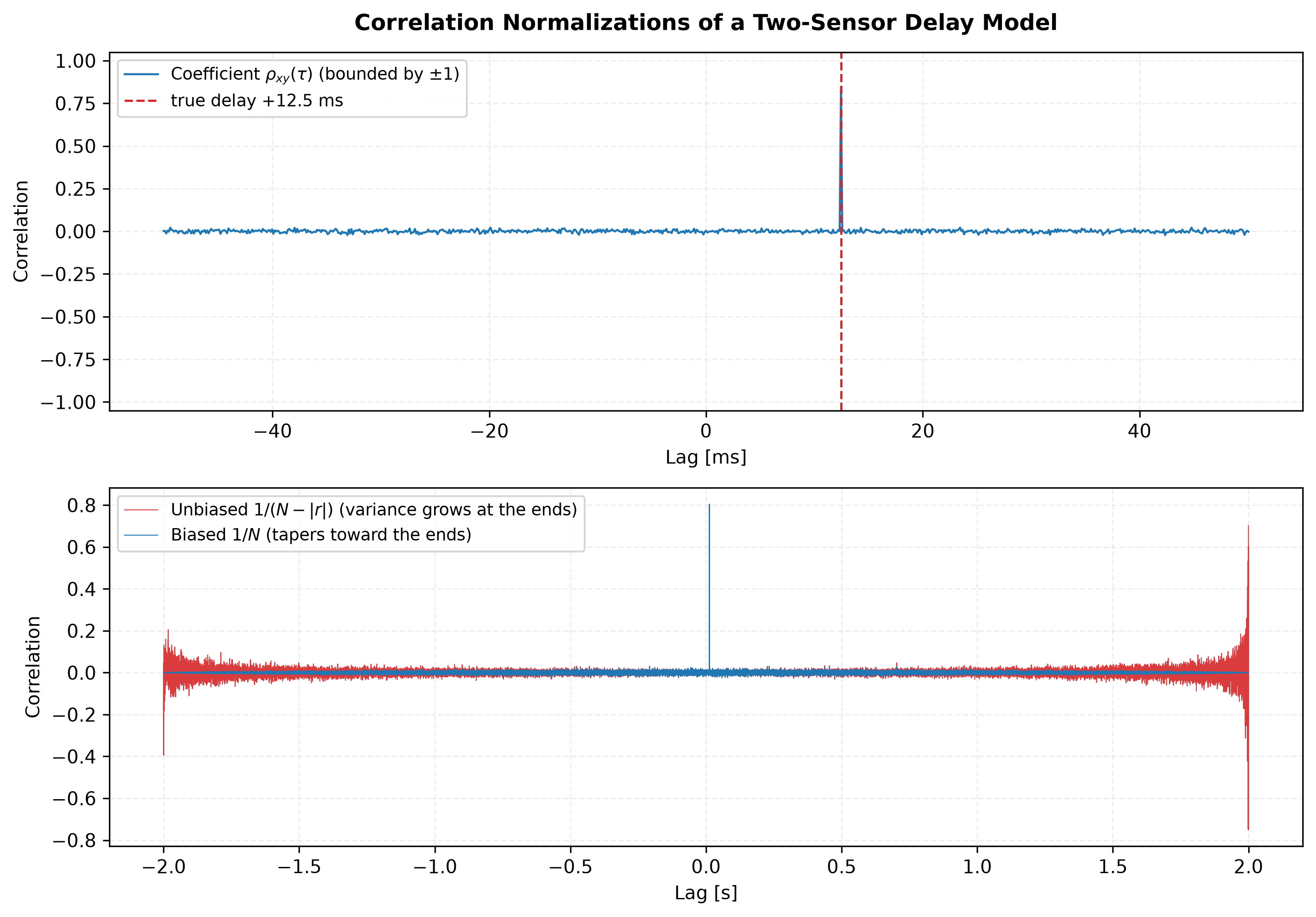

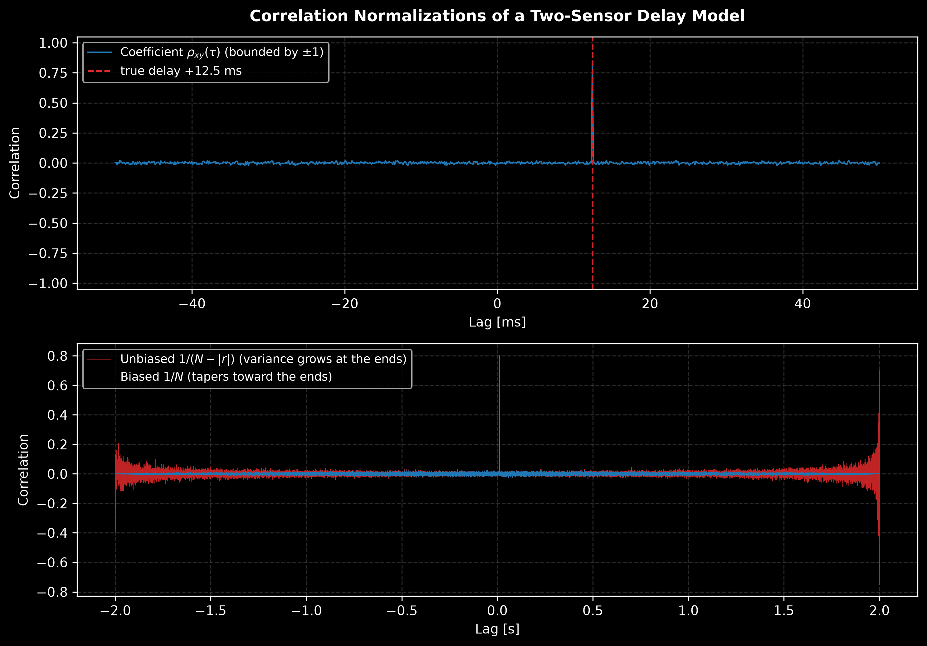
The two-sensor delay model $y(t)=0.8x(t-{\tau }_0)+n(t)$ under the three normalizations: the coefficient function is bounded and peaks at $+{\tau }_0$ (top); over the full lag range the biased estimate tapers toward the ends while the unbiased one pays for its unbiasedness with variance that grows there (bottom).

Show the code for this figure

import matplotlib.pyplot as plt
import numpy as np
from phonometry import correlation, noise_signal

fs = 8192.0
delay = 102                                  # 12.45 ms
x = noise_signal(fs, 2.0, seed=4)
interference = noise_signal(fs, 2.0, rms=0.5, seed=5)
y = 0.8 * np.concatenate([np.zeros(delay), x[:-delay]]) + interference

res = correlation(x, y, fs, normalization="coefficient", max_lag=0.05)

# One line — the correlation estimate against the lag in seconds:
res.plot()
plt.show()

# The three normalizations by hand, from the same records:
biased = correlation(x, y, fs, normalization="biased")
unbiased = correlation(x, y, fs, normalization="unbiased")

fig, (ax_c, ax_n) = plt.subplots(2, 1)
ax_c.plot(1e3 * res.lags, res.values, label="coefficient")
ax_c.axvline(1e3 * delay / fs, color="r", linestyle="--",
             label="true delay")
ax_c.set(xlabel="Lag [ms]", ylabel="Correlation")
ax_n.plot(unbiased.lags, unbiased.values, "r", lw=0.5, label="unbiased")
ax_n.plot(biased.lags, biased.values, lw=0.5, label="biased")
ax_n.set(xlabel="Lag [s]", ylabel="Correlation")
for ax in (ax_c, ax_n):
    ax.legend()
plt.show()

The result always carries the coefficient function alongside the requested normalization, because the coefficient is what the error formulas need. For bandwidth-limited Gaussian data of bandwidth $B$ observed for $T$ seconds (Eqs. 8.109/8.112, valid for $T\ge 10|\tau |$ and $BT\ge 5$):

$$\epsilon \left[{\hat{R}}_{xy}(\tau )\right]=\frac{{\left[1+{\rho }_{xy}^{-2}(\tau )\right]}^{1/2}}{\sqrt{2BT}},\epsilon \left[{\hat{R}}_{xx}(0)\right]=\frac{1}{\sqrt{BT}}.$$

res.random_error(signal_bandwidth) evaluates it per lag with the measured coefficient, and the standalone correlation_random_error takes an explicit coefficient. In the book’s Example 8.5 a common signal of power $S$ reaches two sensors carrying independent noises of power $M$ and $N_2$, so the correlation coefficient at the delay is $\rho =S/\sqrt{(S+M)(S+N_2)}$; with both noises ten times the signal that is $1/11$, and for $B=100$ Hz over $T=5$ s the formula returns $\epsilon \approx 0.35$, one of the pinned conformance anchors — correlation_random_error(1/11, 100.0, 5.0) prints 0.349, which is the whole of Example 8.5 in one call.

($N$ above is the record length in samples, as the normalization bullets use it; the second sensor’s noise power is written $N_2$ here to keep the two apart.) Two closed forms anchor the estimator itself in the tests: the autocorrelation of a sine, $(A^2/2)\cos (2\pi f_0\tau )$, and the $\sin (2\pi B\tau )/(2\pi B\tau )$ autocorrelation of bandwidth-limited white noise (Eq. 8.120).

2. Time-delay estimation

time_delay estimates the delay of $y$ relative to $x$ in the two-sensor model $y(t)=\alpha x(t-{\tau }_0)+n(t)$ (B&P Section 5.1.4) by three routes:

• 'direct': the peak of the full-record correlation coefficient function;
• 'phase': the $|G_{xy}|$-weighted least-squares slope of the cross-spectrum phase (Eq. 5.101b): a pure delay has an exactly linear phase, so this estimator resolves fractional delays to better than 1e-3 samples without any peak interpolation, as long as the unwrapped phase is unambiguous (clean, moderate delays);
• 'gcc': the generalized cross-correlation of Knapp & Carter (1976): the Welch-averaged cross-spectrum is weighted by $\psi (f)$ before the inverse transform, sharpening the peak that the signal’s own autocorrelation would otherwise smear (their Eq. 9).

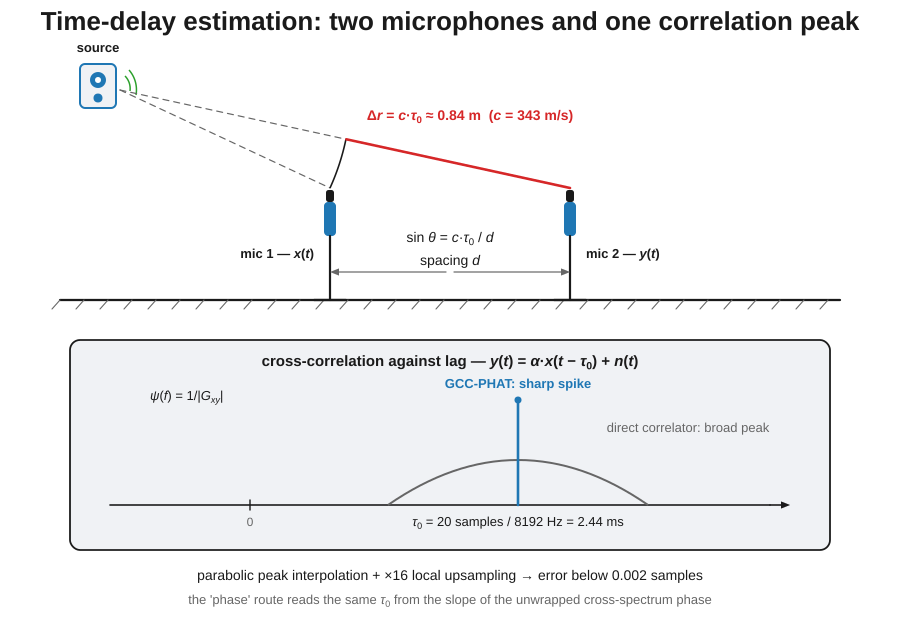
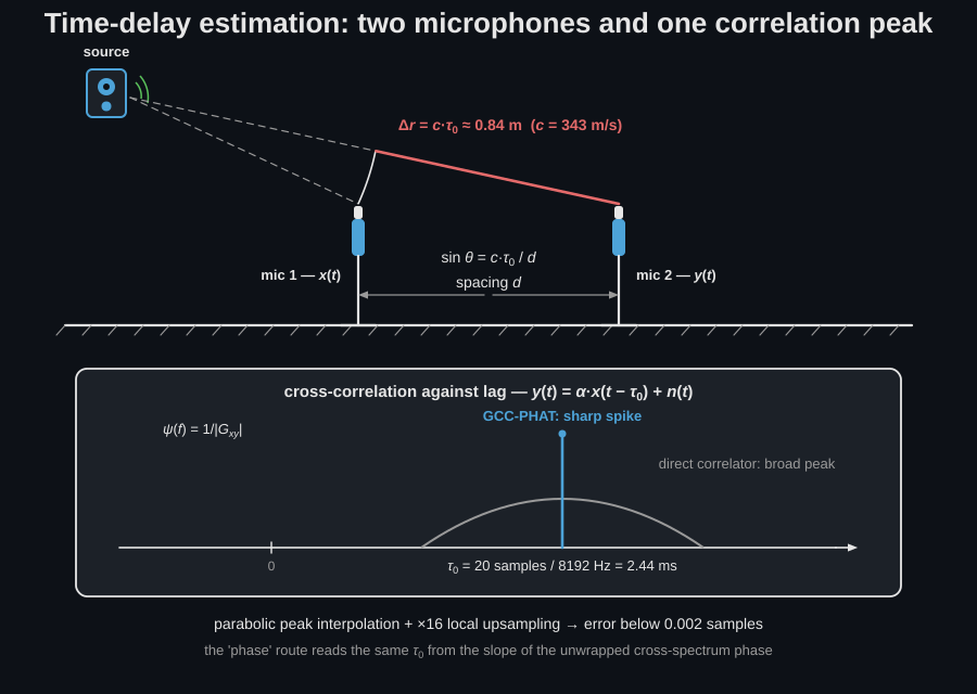
The physical picture is two microphones and one wavefront: the extra path to the far microphone is $c$ times the delay, and the whole estimation problem is locating one peak on the lag axis.

From delay to geometry

A delay is rarely the answer; it is the intermediate. Multiply it by the speed of sound and it becomes a path difference, and for a plane wave arriving at an angle $\theta$ from broadside on a pair spaced $d$ apart,

$$\sin \theta =\frac{c{\tau }_0}{d},$$

so the diagram’s 2.44 ms at 343 m/s is 0.84 m of extra path — a number that only makes sense for a pair spaced at least that far apart. Three limits come with it, and all three are checkable:

• $|c{\tau }_0|>d$ is unphysical. If the estimate exceeds the spacing, the estimator locked onto the wrong peak or onto a reflection. Setting max_delay=d/c keeps the search inside the range the geometry allows, which is the cheapest guard on the page.
• The plane-wave form needs the source in the far field of the pair. Closer than that, wavefront curvature biases $\theta$, and the two microphones see different angles of the same wavefront.
• The angular resolution is worst at endfire. Differentiating, $\mathrm{d}\theta =c\mathrm{d}\tau /(d\cos \theta )$, so a fixed timing uncertainty becomes an ever larger angular error as $\theta$ approaches ±90°, where $\cos \theta \to 0$. A pair is sharp broadside and blind endfire, which is why direction finding uses more than two sensors.

The spacing $d$ therefore fixes both the unambiguous range of the pair and the angular resolution it can offer, and it is the first number to choose when the delay is going to be turned into a direction.

The weightings of Knapp & Carter’s Table I, with the conditions the paper attaches to each:

weighting	$\psi (f)$	Behaviour and conditions
'none'	$1$	The plain correlator: the delta at the delay is convolved with the signal autocorrelation, giving a broad peak on colored signals.
'roth'	$1/G_{xx}$	Suppresses the bands where the first sensor is noisy; still smears unless that noise is spectrally similar to the signal.
'scot'	$1/\sqrt{G_{xx}{G}_{yy}}$	Prewhitens both channels symmetrically; equals Roth when the sensors match.
'phat'	$1/|G_{xy}|$	Ideally a delta at the delay for uncorrelated noises (their Eq. 23), but the weight ignores the signal-to-noise ratio, so bands without signal contribute unit-magnitude random phase. It needs signal power across the analysis band.
'ml'	${\gamma }^2/(|G_{xy}|(1-{\gamma }^2))$	The Hannan-Thomson maximum-likelihood processor: a PHAT weighted down by the phase variance each band actually carries. Attains the Cramér-Rao bound; the safe default when the signal does not fill the band.

Knapp & Carter’s conditions are all written for sensor noise: an anechoic pair with independent noise added at each microphone. The degradation an acoustician meets indoors is different in kind, because a reflection is a coherent copy of the signal rather than noise, and it changes the choice:

• Sensor noise dominates (a quiet room, an outdoor pair, a long baseline): 'ml' is optimal, because it down-weights each band by the phase variance that band actually carries.
• Reverberation dominates (a poor direct-to-reverberant ratio): 'phat' is the standard choice precisely because it discards magnitude, so a strong reflection cannot dominate the peak by being loud.
• Neither converges: window the record around the direct arrival and correlate only the first few milliseconds, which is the only move that removes a reflection rather than reweighting it.

The failure signature is worth memorising, because no returned number reports it: a correlogram whose main peak is not much taller than its neighbours, or a delay that jumps between segments of the same record, means the direct path is not dominant and the delay you have is a reflection’s. delay_std will not warn you — Eq. 8.129 models the scatter of a single peak, not the choice between two.

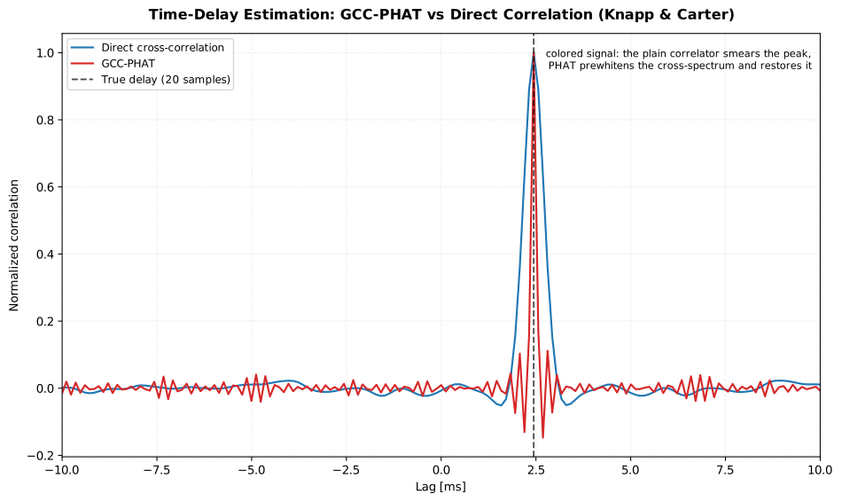
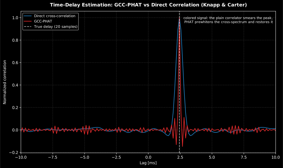
Both estimators land on the 2.441 ms delay — 2.4413 ms direct, 2.4418 ms PHAT — so the argument is not about accuracy on a clean pair but about how much the peak can be trusted. Prewhitening narrows the main lobe from 0.73 ms at half height to 0.24 ms, two samples at 8192 Hz, because the direct correlator convolves the delta with the autocorrelation of a signal that is band-limited to 800 Hz while PHAT throws that magnitude away. Read the width, not the position: it is what says whether a reflection could be sitting under the peak.

Show the code for this figure

import matplotlib.pyplot as plt
import numpy as np
from scipy import signal as sp_signal
from phonometry import noise_signal, time_delay

fs = 8192.0
delay = 20  # samples
b, a = sp_signal.butter(2, 800.0 / (fs / 2.0))   # colored common signal
s = sp_signal.lfilter(b, a, noise_signal(fs, 4.0, color="white", seed=10))
x = s + noise_signal(fs, 4.0, color="white", rms=0.02, seed=11)
y = np.roll(s, delay) + noise_signal(fs, 4.0, color="white", rms=0.02, seed=12)

direct = time_delay(x, y, fs, method="direct", max_delay=0.01)
phat = time_delay(x, y, fs, method="gcc", weighting="phat",
                  nperseg=2048, max_delay=0.01)

fig, ax = plt.subplots(figsize=(10, 6))
ax.plot(1e3 * direct.lags,
        direct.correlation / np.max(np.abs(direct.correlation)),
        label="Direct cross-correlation")
ax.plot(1e3 * phat.lags, phat.correlation, label="GCC-PHAT")
ax.axvline(1e3 * delay / fs, ls="--", color="k", label="True delay")
ax.set_xlabel("Lag [ms]")
ax.set_ylabel("Normalized correlation")
ax.legend()
plt.show()

The correlation-peak methods refine the sample peak by three-point parabolic interpolation, optionally after band-limited local upsampling (upsample=16 resamples a window around the peak sixteenfold before the parabola). Sub-sample accuracy presumes the peak is oversampled, i.e. the signals are band-limited below Nyquist; on a $0.4f_s$ band-limited pair the tests pin the achievable error at ≲0.1 sample for the parabola alone and ≲2e-3 samples with upsample=16. For GCC the delay must fit within half a Welch segment; raise nperseg for longer delays.

With signal_bandwidth given, the result also carries the peak-location uncertainty of B&P Eq. 8.129 and its $\pm 2\sigma$ interval (Eq. 8.130):

$$\sigma ({\hat{\tau }}_0)\approx {\left(\frac{3}{4}\right)}^{1/4}\frac{\sqrt{\epsilon [{\hat{R}}_{xy}({\tau }_0)]}}{\pi B}.$$

from phonometry import time_delay

res = time_delay(x, y, fs, method="gcc", weighting="ml",
                 nperseg=2048, upsample=16, signal_bandwidth=1000.0)
print(res.delay, res.delay_samples)     # seconds and fractional samples
print(res.delay_std, res.delay_interval)  # Eq. 8.129 sigma, +/-2 sigma
res.plot()                              # correlation with the delay marked

The formula models the peak of the continuous correlation function, so treat the interval as a conservative order-of-magnitude bound; the seeded Monte Carlo in the test suite observes the actual scatter below the prediction.

3. Impulse-response delay and alignment

The cross-correlation of an impulse response with an ideal unit impulse is the IR itself, so the sub-sample location of its peak magnitude is its arrival time. impulse_response_delay applies exactly the same refinement as the TDE peak (local band-limited upsampling, default ×8, plus the parabola), and with a reference IR it measures the delay between the pair from their full-record cross-correlation (one-shot transients are not stationary records, so the direct correlator is used rather than the Welch-averaged GCC):

from phonometry import align_impulse_responses, impulse_response_delay

t_arrival = impulse_response_delay(ir, fs)              # seconds from t = 0
dt = impulse_response_delay(ir_b, fs, reference=ir_a)   # pair delay

res = align_impulse_responses(ir_b, ir_a, fs)  # remove the estimated delay
res.plot()                                     # reference vs aligned overlay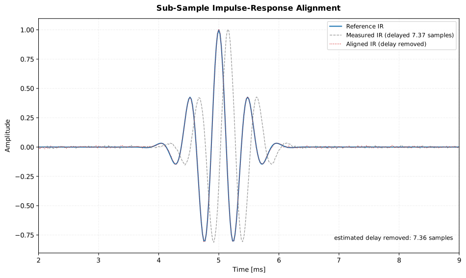

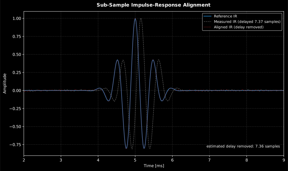
A measured IR delayed by a fractional 7.37 samples (dashed) is aligned back onto its reference: the band-limited shift removes the estimated 7.36 samples and the aligned trace (dotted) lands on the reference.

Show the code for this figure

import matplotlib.pyplot as plt
import numpy as np
from scipy import signal as sp_signal
from phonometry import align_impulse_responses, fractional_delay

fs = 48000.0
t = np.arange(int(0.03 * fs)) / fs
rng = np.random.default_rng(6)
# Band-limited reference pulse: a 2 kHz Gaussian tone burst at 5 ms.
ir_a = sp_signal.gausspulse(t - 0.005, fc=2000.0, bw=0.5)
ir_b = fractional_delay(ir_a, 7.37)[: ir_a.size]
ir_b += 0.005 * rng.standard_normal(ir_a.size)

res = align_impulse_responses(ir_b, ir_a, fs)

# One line — reference and aligned IR overlaid:
res.plot()
plt.show()

# By hand, from the fields the result carries:
t_ms = 1e3 * t
fig, ax = plt.subplots()
ax.plot(t_ms, res.reference, lw=1.6, label="Reference IR")
ax.plot(t_ms, ir_b, "0.5", lw=1.0, linestyle="--", label="Measured IR")
ax.plot(t_ms, res.aligned[: t.size], "r:", label="Aligned IR")
ax.set(xlabel="Time [ms]", ylabel="Amplitude",
       title=f"delay removed: {res.delay_samples:.2f} samples")
ax.legend()
plt.show()

align_impulse_responses removes the estimated delay with an exact band-limited fractional shift (a frequency-domain phase ramp over a zero-padded record, so nothing wraps around): the tool for averaging IR ensembles or comparing measurements taken at slightly different distances. The synthetic fractional-delay tests document the achievable accuracy on a smooth band-limited pulse: about 1e-2 samples with the parabola alone, 1e-3 at the default upsample=8, below 1e-5 at ×32.

4. Hilbert envelope and instantaneous frequency

envelope builds the analytic signal $z(t)=x(t)+j\tilde{x}(t)$ by the one-sided spectrum construction that Bendat & Piersol recommend (Eq. 13.25) and returns the three Chapter 13 quantities on one time axis:

$$A(t)={\left[x^2(t)+{\tilde{x}}^2(t)\right]}^{1/2},\theta (t)=\arctan \frac{\tilde{x}(t)}{x(t)},f(t)=\frac{1}{2\pi }\frac{d\theta }{dt}.$$

These three are physically meaningful only if the record really is one carrier with a slow modulation: the modulation bandwidth has to stay below the carrier frequency, so that the two spectra do not overlap. That is the narrowband (Bedrosian) condition, and it is exactly why the exact AM identity below holds. Nothing in the call enforces it — envelope returns numbers for any array you hand it.

A violation is easy to recognise once you know what to look for. The envelope stops being smooth and starts tracking individual half-cycles of the waveform, and the instantaneous frequency spikes, leaves the signal’s band entirely and goes negative — which happens every time the analytic signal passes near the origin of the complex plane, and is a geometric artefact rather than a physical frequency. Applied to speech, to a room impulse response or to broadband noise, all three quantities do this. The fix is to make the record narrowband first: band-pass around the component of interest, exactly as the envelope spectrum does with its band= front end, or read the ridge of a spectrogram when several components coexist — the Hilbert construction has no way to represent more than one at a time.

For an amplitude-modulated carrier $u(t)\cos (2\pi f_{0}t)$ the envelope recovers $u(t)$ exactly (Eq. 13.27); the conformance suite pins the recovered AM envelope and the Table 13.1 pair $\cos \to \sin$ at the 1e-9 level, and the instantaneous frequency of a chirp tracks its sweep.

from phonometry import envelope

res = envelope(x, fs)
print(res.envelope, res.instantaneous_frequency)
res.plot()               # signal + envelope, instantaneous frequency

slow = envelope(x, fs, decimation_factor=32)   # anti-aliased, fs/32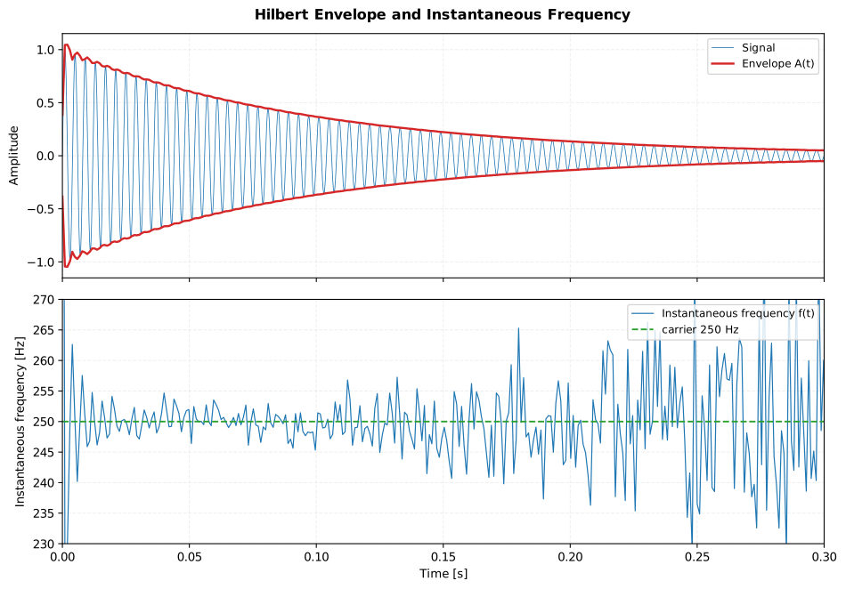

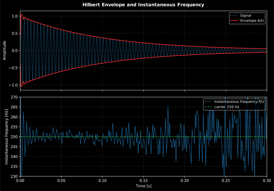
The Hilbert quantities of a struck 250 Hz mode: the envelope traces the exponential decay (top), and the instantaneous frequency sits on the carrier while the mode dominates, jittering as the signal sinks into the noise floor (bottom, ×8 anti-aliased decimation).

Show the code for this figure

import matplotlib.pyplot as plt
import numpy as np
from phonometry import envelope

fs = 8192.0
t = np.arange(int(0.4 * fs)) / fs
rng = np.random.default_rng(7)
x = np.exp(-t / 0.1) * np.sin(2 * np.pi * 250.0 * t)   # a struck mode
x += 0.001 * rng.standard_normal(t.size)

res = envelope(x, fs, decimation_factor=8)

# One line — signal + envelope and the instantaneous frequency:
res.plot()
plt.show()

# By hand, from the fields the result carries:
fig, (ax_e, ax_f) = plt.subplots(2, 1, sharex=True)
ax_e.plot(t, res.signal, lw=0.6, label="Signal")
ax_e.plot(res.times, res.envelope, "r", lw=1.8, label="Envelope A(t)")
ax_e.plot(res.times, -res.envelope, "r", lw=1.8)
ax_e.legend()
ax_f.plot(res.times, res.instantaneous_frequency, lw=0.9,
          label="Instantaneous frequency f(t)")
ax_f.axhline(250.0, color="g", linestyle="--", label="carrier 250 Hz")
ax_f.set(xlabel="Time [s]", ylabel="Frequency [Hz]", ylim=(230, 270))
ax_f.legend()
plt.show()

The envelope of a band-limited signal is itself low-frequency, so the result offers optional decimation: a zero-phase FIR anti-alias filter by default, or plain subsampling with antialias=False, exactly the convention the ECMA-418-2 loudness/roughness chain of phonometry.psychoacoustics applies internally after its auditory bandpass (Formulae 65/119 of the standard), appropriate when the input is already narrowband.

Relation to the spectral estimators

time_delay (GCC and phase methods) runs on the same Welch core (taper, overlap policy, detrend-off calibration, segment defaults) as cross_spectral_density and the H1/H2 frequency-response estimators, so a GCC, a coherence and a cross-spectrum computed with the same segment length agree bin by bin; the 'phase' estimator is literally the slope of the CrossSpectralDensityResult phase, weighted as Eq. 5.101b prescribes.

The Hilbert envelope here is the time-domain companion of the envelope spectrum, which reads the same modulations off as discrete lines in frequency; and the sub-sample alignment shares its band-limited kernel with the public fractional-delay and resampling tools.

What this guide covers

• Covered

  Bendat & Piersol Chapter 5, Section 8.4 and Chapter 13: correlation with the biased, unbiased and coefficient normalizations and their random-error formulas (Eqs. 8.109/8.112); time_delay with the direct, phase-slope and Knapp & Carter (1976) generalized cross-correlation methods, including the Roth, SCOT, PHAT and maximum-likelihood weightings of their Table I; the peak-location uncertainty of Eq. 8.129; impulse_response_delay and align_impulse_responses; and the Hilbert envelope with instantaneous phase and frequency (Chapter 13).

• Not covered

  correlation and time_delay model a single common-path delay between exactly two sensors (the $y(t)=\alpha x(t-{\tau }_0)+n(t)$ model of Eq. 5.21). A record with several arrivals (multipath, a direct path plus reflections) is not separated automatically: time_delay and the direct correlator report only the single largest peak, the same limitation echo_detection names on the cepstrum in Cepstrum, echoes and the envelope spectrum. Estimating delays across more than two sensors, as an array or beamformer would, means calling these pairwise functions yourself; there is no built-in multi-sensor TDOA solver.

See also

• Cepstrum, echoes and the envelope spectrum: the reference-free route to a delay, and the envelope this page constructs.
• Calibrated spectral analysis: the cross-spectrum the GCC weightings are built from, and the two-channel acquisition rules.
• Test signals: the band-limited fractional-delay kernel behind the sub-sample alignment.
• Time synchronous averaging: the same alignment applied per revolution.
• API reference: signals.correlation and signals.envelope.

References

• Bendat, J. S., & Piersol, A. G. (2010). Random data: Analysis and measurement procedures (4th ed.). Wiley. https://doi.org/10.1002/9781118032428Sections 5.1.4 and 5.2.6-5.2.7 (time delay via correlation and cross-spectrum), 8.4 (random errors of correlation estimates and of the peak location), 11.4 (FFT computation with zero padding) and Chapter 13 (Hilbert transforms, envelope and instantaneous phase). ISBN 978-0-470-24877-5.
• Knapp, C. H., & Carter, G. C. (1976). The generalized correlation method for estimation of time delay. IEEE Transactions on Acoustics, Speech, and Signal Processing, 24(4), 320-327. https://doi.org/10.1109/TASSP.1976.1162830The GCC framework, the Table I weightings and their conditions, and the maximum-likelihood (Hannan-Thomson) processor.