Filter Architecture Gallery

Choosing a filter architecture is a trade-off: selectivity, passband ripple and phase behaviour cannot all be optimal at once, and each of the five architectures phonometry offers resolves the trade-off differently. Three of them — Butterworth, Chebyshev II and Bessel — place their −3 dB points on the ANSI S1.11 band edges, so for those three the choice changes how a band rejects its neighbours and how it treats transients, not where the band sits. The two equiripple designs are the exception, and section 3 gives the size of it: cheby1 and ellip treat the band edges as their ripple edge, so their bands are effectively wider and every band level reads a few tenths of a decibel high. This page puts the architectures side by side: the comparison at the −3 dB crossover, the full 1/1 and 1/3 octave response gallery, usage examples per architecture, and the Linkwitz-Riley crossover for when the goal is splitting a signal rather than measuring bands.

The design mathematics behind these banks (band edges, poles and zeros, multirate decimation) and the parameter reference live in Filter Banks; proving that a designed bank meets a performance class of IEC 61260-1 is Filter Class Verification.

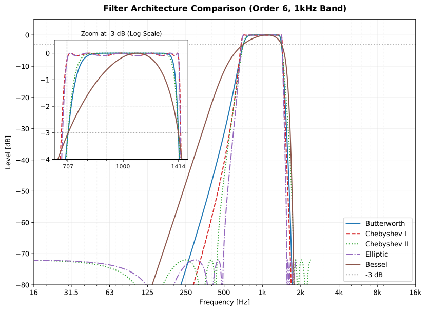
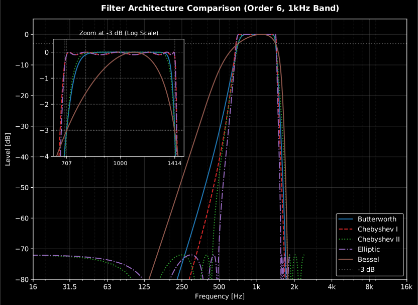
1. The five architectures at the band edges

All five designs are compared on the same 1 kHz octave band at 48 kHz. Read the figure twice: the wide view shows how fast each skirt falls away from the band, and the inset around the −3 dB line shows where they cross. What changes between those two views is that Chebyshev I ripples inside the band, Chebyshev II ripples outside it, Elliptic does both and falls fastest, and Bessel is the smoothest and the slowest.

Show the code for this figure

import matplotlib.pyplot as plt
import numpy as np
from scipy.signal import sosfreqz
from phonometry import filters

fs = 48000
fig, ax = plt.subplots(figsize=(9, 5))
for ftype in ("butter", "cheby1", "cheby2", "ellip", "bessel"):
    # limits picks out the single 1 kHz octave band
    bank = filters.OctaveFilterBank(fs, fraction=1, order=6, limits=[800, 1200],
                            design=filters.FilterDesign(filter_type=ftype))
    idx = int(np.argmin(np.abs(np.array(bank.freq) - 1000)))
    fsd = fs / bank.factor[idx]           # rate the band actually runs at
    w, h = sosfreqz(bank.sos[idx], worN=16384, fs=fsd)
    ax.semilogx(w, 20 * np.log10(np.abs(h) + 1e-9), label=ftype)
ax.axhline(-3, color="gray", linestyle=":", label="-3 dB")

# The inset the section is named after: the same curves around the crossover.
from mpl_toolkits.axes_grid1.inset_locator import inset_axes

axins = inset_axes(ax, width="35%", height="45%", loc="upper left", borderpad=3)
for line in ax.get_lines()[:-1]:
    axins.semilogx(line.get_xdata(), line.get_ydata(), label=line.get_label())
axins.axhline(-3, color="gray", linestyle=":")
axins.set(xscale="log", xlim=(650, 1500), ylim=(-4, 0.5),
          title="Zoom at -3 dB (log scale)")

ax.set(xlim=(100, 8000), ylim=(-80, 5),
       xlabel="Frequency [Hz]", ylabel="Magnitude [dB]")
ax.grid(True, which="both", alpha=0.3)
ax.legend()
plt.show()

Type	Name	Usage Example	Best For
butter	Butterworth	octave_filter(x, fs, design=FilterDesign(filter_type='butter'))	General acoustic measurement.
cheby1	Chebyshev I	octave_filter(x, fs, design=FilterDesign(filter_type='cheby1', ripple=0.1))	Sharper roll-off at the cost of ripple.
cheby2	Chebyshev II	octave_filter(x, fs, design=FilterDesign(filter_type='cheby2'))	Flat passband with stopband zeros.
ellip	Elliptic	octave_filter(x, fs, design=FilterDesign(filter_type='ellip', ripple=0.1))	Maximum selectivity.
bessel	Bessel	octave_filter(x, fs, design=FilterDesign(filter_type='bessel'))	Preserving transient waveform shapes (see the group-delay figure of Filter Banks).

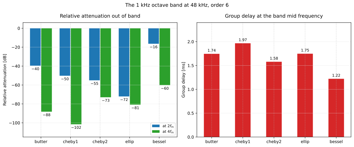
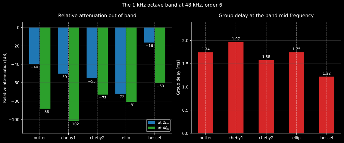
The choice, quantified. Selectivity and group delay move in opposite directions, and the class column of the table below says which of the five you may actually use for a standards-compliant band measurement.

Architecture	Ripple across the band centre	At $2f_m$	At $4f_m$	Group delay at $f_m$	IEC 61260-1 class (order 6, 48 kHz)
butter	0.00 dB	−39.6 dB	−88.2 dB	1.74 ms	1
cheby1	0.10 dB	−50.2 dB	−101.6 dB	1.97 ms	none
cheby2	0.00 dB	−55.1 dB	−73.0 dB	1.58 ms	1
ellip	0.10 dB	−72.1 dB	−80.8 dB	1.75 ms	none
bessel	0.21 dB	−16.4 dB	−60.2 dB	1.22 ms	none

Read the last column first: three of the five cannot be used for a standards-compliant band measurement at all with the default parameters — the equiripple pair because their band edges are not their −3 dB points (see Filter Banks), Bessel because it rolls off too slowly for the mask. That is a hard constraint, not a preference, and it comes before any of the other columns. Among the two that pass, the choice is a real trade: cheby2 buys 15 dB more rejection one octave out and pays for it with a 15 dB shallower far stopband, because its equiripple floor is pinned at attenuation.

One more thing the table cannot show: rejection only matters when a strong neighbour must not contaminate a weak band, and there the ceiling is the attenuation parameter (72 dB by default), not the architecture.

Show the code for this figure

import numpy as np
from scipy.signal import sosfreqz

# `filters` is the import of the snippet above.
fs = 48000
for ftype in ("butter", "cheby1", "cheby2", "ellip", "bessel"):
    # resample=False so the response exists above the decimated Nyquist
    bank = filters.OctaveFilterBank(
        fs, fraction=1, order=6, limits=[800, 1200],
        design=filters.FilterDesign(filter_type=ftype, resample=False))
    idx = int(np.argmin(np.abs(np.array(bank.freq) - 1000)))
    f_m = float(bank.freq[idx])
    w, h = sosfreqz(bank.sos[idx], worN=1 << 17, fs=fs)
    mag = 20 * np.log10(np.abs(h) + 1e-15)
    mag -= mag.max()

    grid = np.linspace(f_m * 0.95, f_m * 1.05, 4001)
    _, h_c = sosfreqz(bank.sos[idx], worN=2 * np.pi * grid / fs)
    delay = -np.gradient(np.unwrap(np.angle(h_c)), 2 * np.pi * grid)

    banked = filters.OctaveFilterBank(
        fs, fraction=1, order=6, limits=[800, 1200],
        design=filters.FilterDesign(filter_type=ftype))
    print(f"{ftype:8s} {mag[np.argmin(abs(w - 2 * f_m))]:7.1f} dB "
          f"{mag[np.argmin(abs(w - 4 * f_m))]:7.1f} dB "
          f"{delay[len(delay) // 2] * 1e3:5.2f} ms "
          f"class {filters.verify_filter_class(banked)['overall_class']}")

2. Gallery of Filter Bank Responses

Full spectral view of the filter banks for Octave (1/1) and 1/3-Octave fractions.

Architecture	Octave (fraction=1)	One-third octave (fraction=3)
Butterworth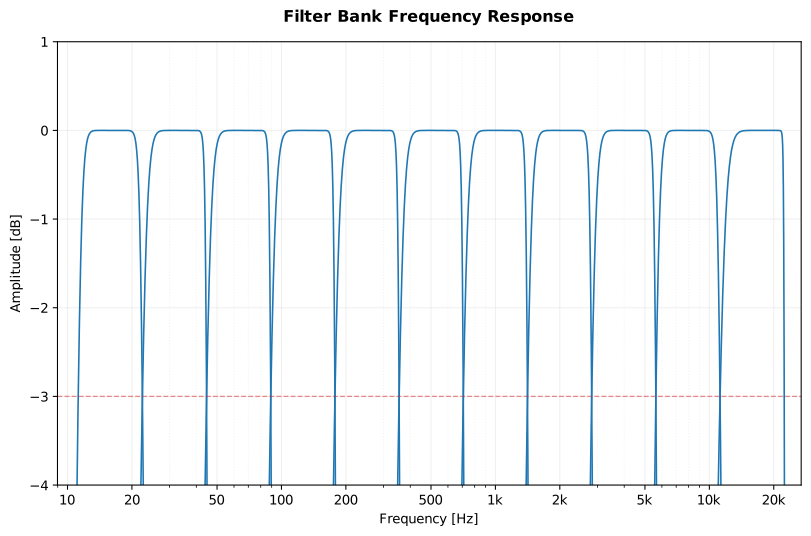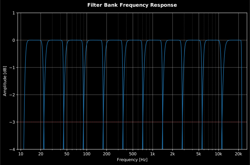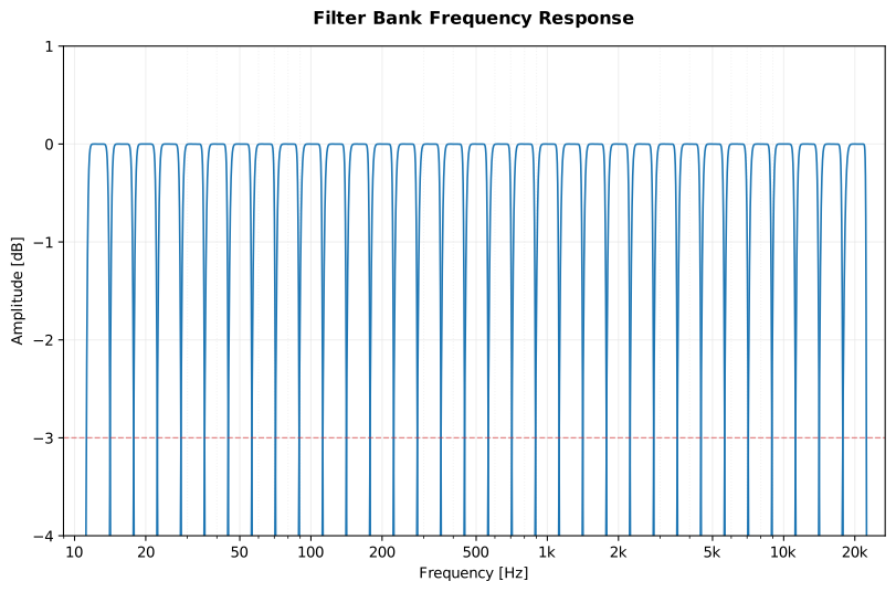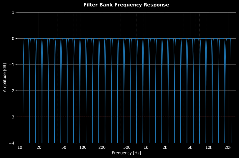
Chebyshev I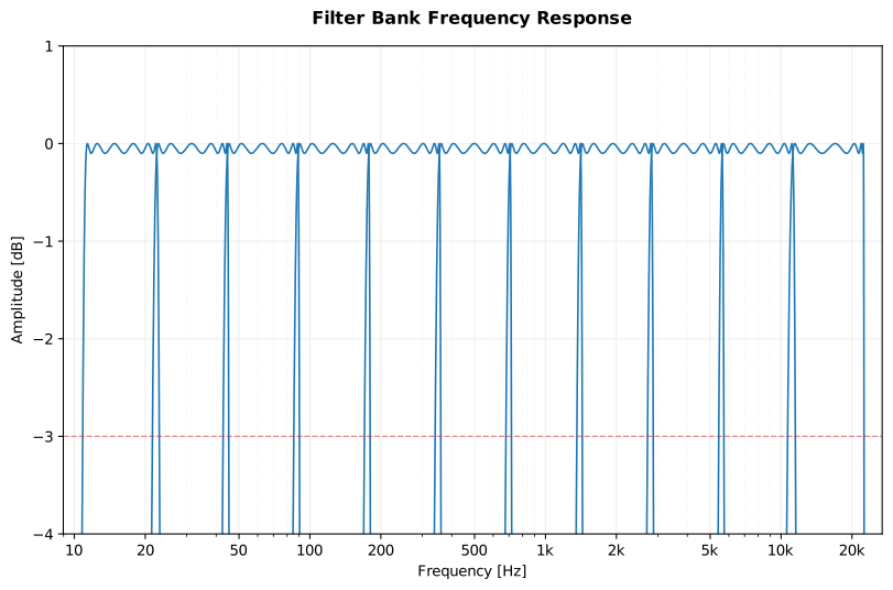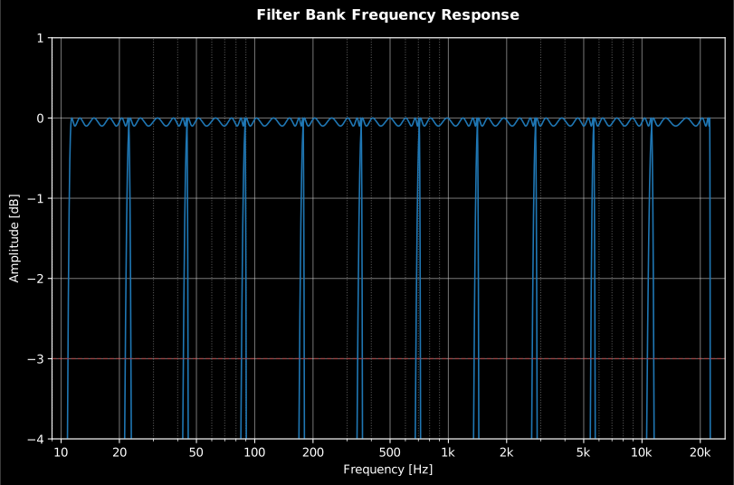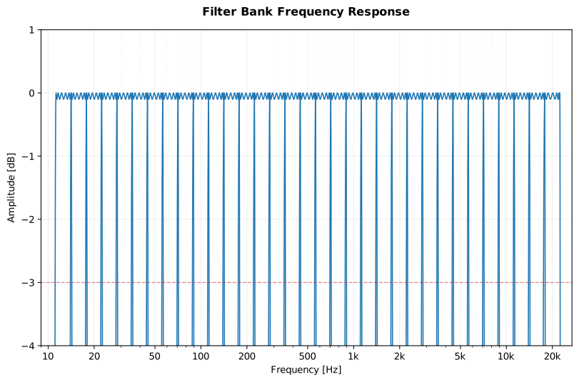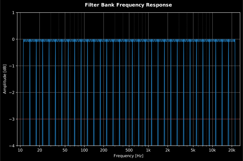
Chebyshev II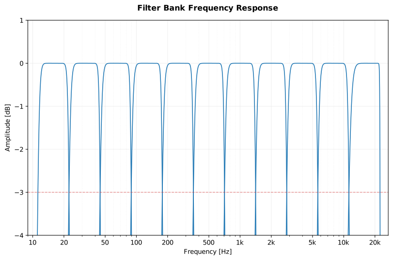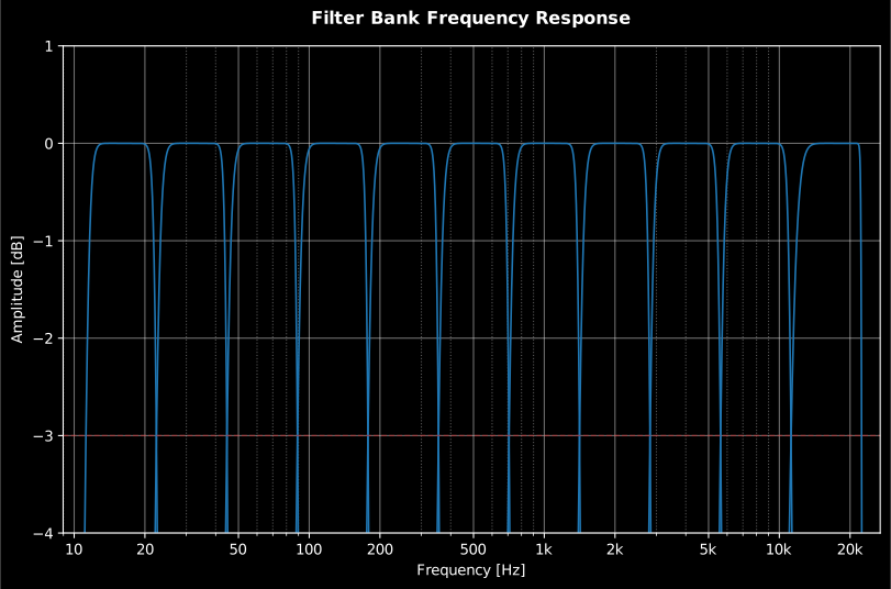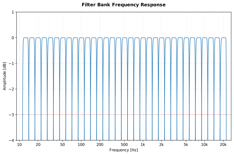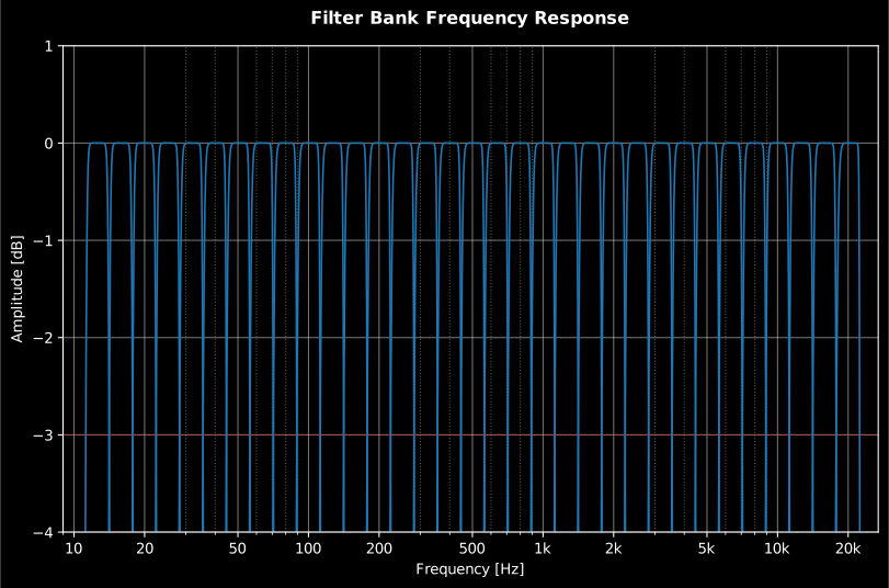
Elliptic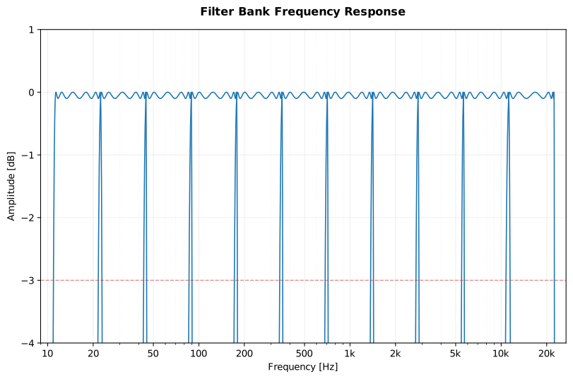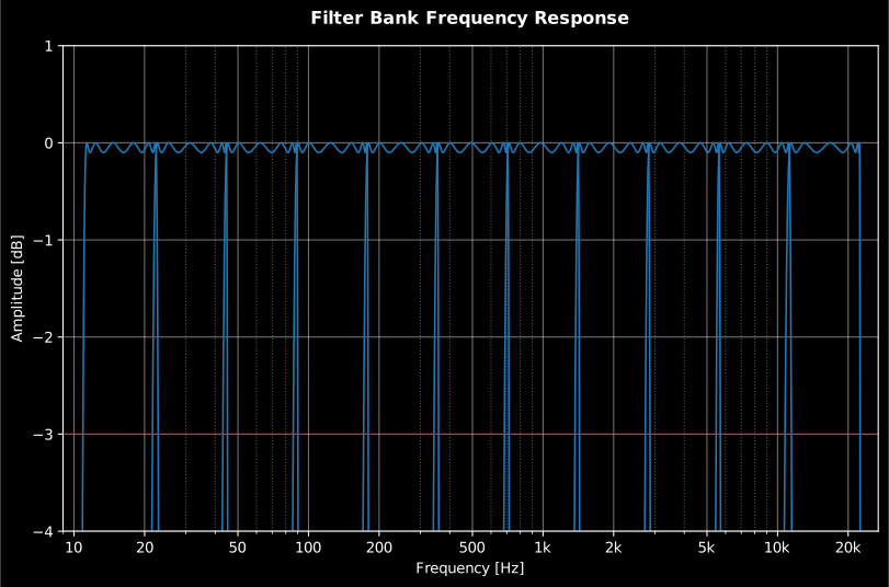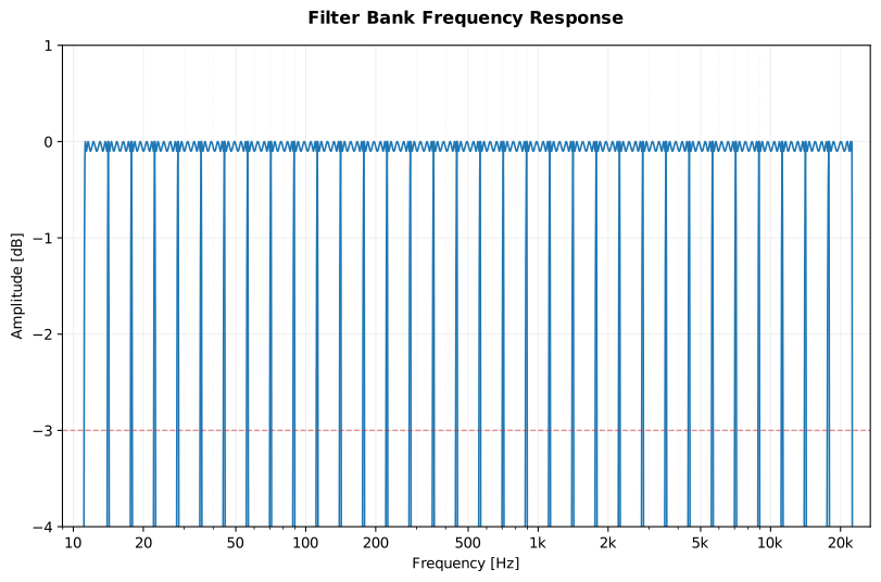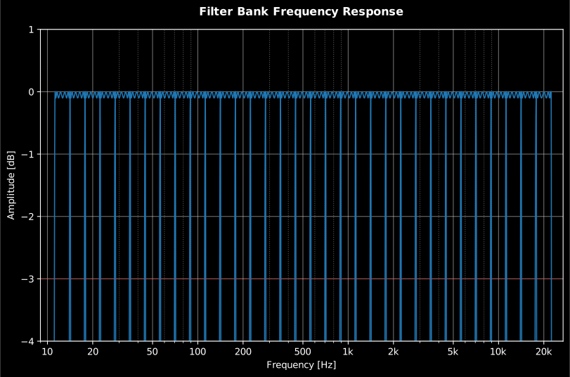
Bessel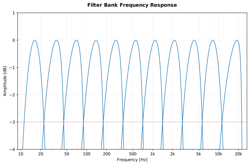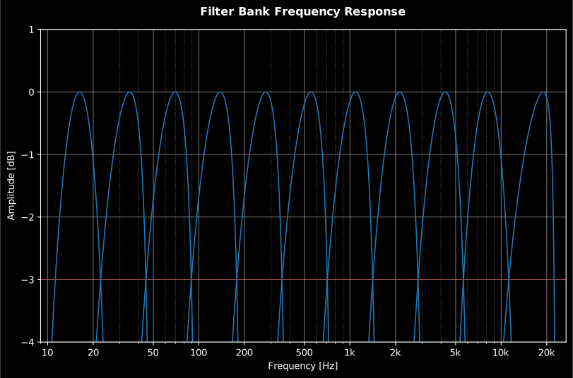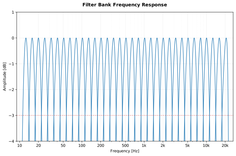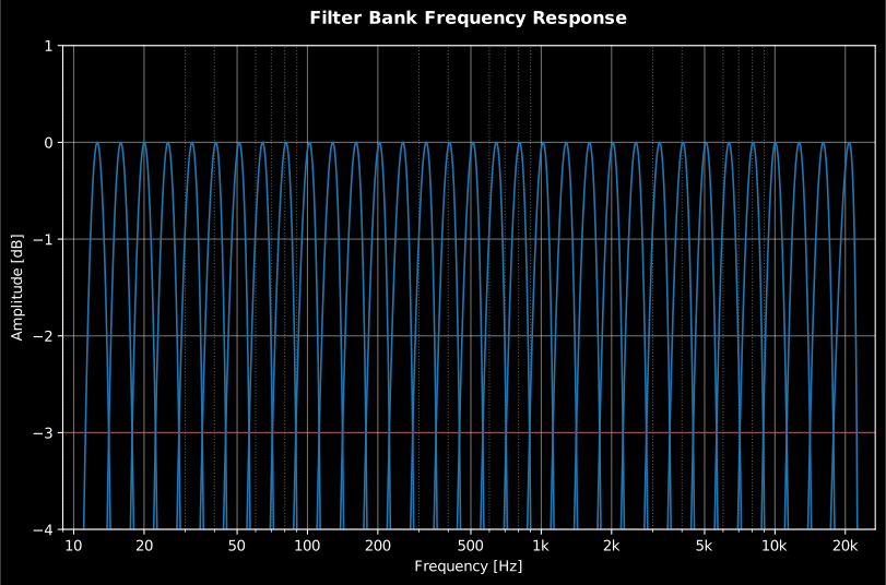

Compare the rows on two things only, and the differences stop being subtle. Flat tops: Chebyshev I puts its ripple inside each band, on the flat top; Chebyshev II puts it outside, as the notch train between bands; Elliptic does both. Valley depth: how far the response falls between two adjacent bands is the leakage budget of a band level, and Bessel’s skirts overlap far more than any of the others — that overlap is its slow roll-off, drawn.

Show the code for this figure

from phonometry import filters

# One figure per architecture and fraction: the whole response gallery
fs = 48000
for ftype in ("butter", "cheby1", "cheby2", "ellip", "bessel"):
    for fraction in (1, 3):
        # ResponsePlot(show=True) draws the bank's frequency response
        filters.OctaveFilterBank(fs=fs, fraction=fraction, order=6,
                                   limits=[12, 20000],
                                   design=filters.FilterDesign(filter_type=ftype),
                                   response_plot=filters.ResponsePlot(show=True))

3. Filter Usage and Examples

1. Butterworth (butter)

The Butterworth filter is known for its maximally flat passband. It is the standard choice for acoustic measurements where no ripple is allowed within the frequency bands.

import numpy as np
from phonometry import filters

# A calibrated signal in Pa so the guide runs standalone
fs = 48000
x = 0.2 * np.sin(2 * np.pi * 1000 * np.arange(fs) / fs)

# Standard one-third-octave measurement
spl, freq = filters.octave_filter(x, fs, fraction=3,
                                  design=filters.FilterDesign(filter_type='butter'))

Show the code for this figure

from phonometry import filters

# Draw this bank's response (1/3 octave, order 6, Butterworth)
filters.OctaveFilterBank(fs=48000, fraction=3, order=6, limits=[12, 20000],
                           design=filters.FilterDesign(filter_type='butter'),
                           response_plot=filters.ResponsePlot(show=True))

2. Chebyshev I (cheby1)

Chebyshev Type I filters provide a steeper roll-off than Butterworth at the expense of ripples in the passband. Useful when high selectivity is needed near the cut-off frequencies.

import numpy as np
from phonometry import filters

# A calibrated signal in Pa so the guide runs standalone
fs = 48000
x = 0.2 * np.sin(2 * np.pi * 1000 * np.arange(fs) / fs)

# Selectivity with 0.1 dB passband ripple
spl, freq = filters.octave_filter(
    x, fs, fraction=3,
    design=filters.FilterDesign(filter_type='cheby1', ripple=0.1))

Show the code for this figure

from phonometry import filters

# Draw this bank's response (1/3 octave, order 6, Chebyshev I)
filters.OctaveFilterBank(fs=48000, fraction=3, order=6, limits=[12, 20000],
                           design=filters.FilterDesign(filter_type='cheby1', ripple=0.1),
                           response_plot=filters.ResponsePlot(show=True))

3. Chebyshev II (cheby2)

Also known as Inverse Chebyshev, it has a flat passband and ripples in the stopband. It provides faster roll-off than Butterworth without affecting the signal in the passband. The stopband edges are placed automatically so that the −3 dB points land on the band edges (attenuation must be $>3.01\text{dB}$ for a −3 dB point to exist at all; below that the design raises ValueError). Note that the default of 72 dB is set by conformance and not by realizability: SciPy pins the equiripple floor at exactly attenuation, and IEC 61260-1 class 1 demands 70 dB far from the band, so an attenuation of, say, 6 dB is arithmetically legal and silently loses the class — see Filter Class Verification.

import numpy as np
from phonometry import filters

# A calibrated signal in Pa so the guide runs standalone
fs = 48000
x = 0.2 * np.sin(2 * np.pi * 1000 * np.arange(fs) / fs)

# Flat passband, class-1 default 72 dB stopband attenuation
spl, freq = filters.octave_filter(x, fs, fraction=3,
                                  design=filters.FilterDesign(filter_type='cheby2'))

Show the code for this figure

from phonometry import filters

# Draw this bank's response (1/3 octave, order 6, Chebyshev II)
filters.OctaveFilterBank(fs=48000, fraction=3, order=6, limits=[12, 20000],
                           design=filters.FilterDesign(filter_type='cheby2'),
                           response_plot=filters.ResponsePlot(show=True))

4. Elliptic (ellip)

Elliptic (Cauer) filters have the shortest transition width (steepest roll-off) for a given order. They feature ripples in both the passband and stopband.

import numpy as np
from phonometry import filters

# A calibrated signal in Pa so the guide runs standalone
fs = 48000
x = 0.2 * np.sin(2 * np.pi * 1000 * np.arange(fs) / fs)

# Maximum selectivity for extreme band isolation
spl, freq = filters.octave_filter(
    x, fs, fraction=3,
    design=filters.FilterDesign(filter_type='ellip', ripple=0.1))

Show the code for this figure

from phonometry import filters

# Draw this bank's response (1/3 octave, order 6, Elliptic)
filters.OctaveFilterBank(fs=48000, fraction=3, order=6, limits=[12, 20000],
                           design=filters.FilterDesign(filter_type='ellip', ripple=0.1),
                           response_plot=filters.ResponsePlot(show=True))

5. Bessel (bessel)

Bessel filters are optimized for linear phase response and minimal group delay. They preserve the shape of filtered waveforms (transients) better than any other type, but have the slowest roll-off. That claim is temporal, so the evidence for it is temporal too, and it lives on the sibling page: the group-delay figure of Filter Banks shows Bessel staying nearly flat across the passband while Chebyshev I and Elliptic peak at the band edges, and the band-decomposition figure of the same page shows what a longer ring does to a transient.

import numpy as np
from phonometry import filters

# A calibrated signal in Pa so the guide runs standalone
fs = 48000
x = 0.2 * np.sin(2 * np.pi * 1000 * np.arange(fs) / fs)

# Best for pulse analysis and transient preservation
spl, freq = filters.octave_filter(x, fs, fraction=3,
                                  design=filters.FilterDesign(filter_type='bessel'))

Show the code for this figure

from phonometry import filters

# Draw this bank's response (1/3 octave, order 6, Bessel)
filters.OctaveFilterBank(fs=48000, fraction=3, order=6, limits=[12, 20000],
                           design=filters.FilterDesign(filter_type='bessel'),
                           response_plot=filters.ResponsePlot(show=True))

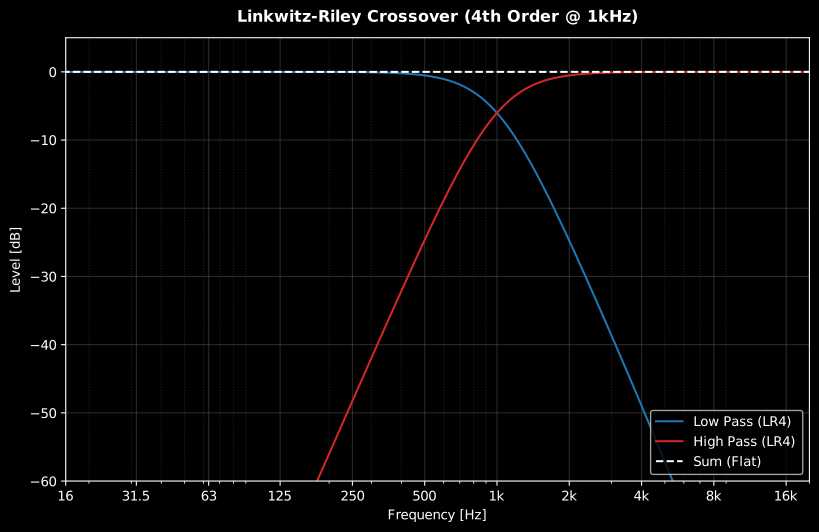
4. Linkwitz-Riley crossover (linkwitz_riley)

Linkwitz-Riley is not a sixth architecture: it does not build an IEC band, and it is not a FilterDesign(filter_type=…) value. It is called directly, and it does the opposite job — it splits one signal into two branches that recombine into a flat magnitude response, which is what a loudspeaker crossover needs and what a measurement band must never do. Each branch is a Butterworth of order order/2 applied twice, so each is exactly −6 dB at the crossover frequency (not −3 dB as in the bands above): the branches add to unity in amplitude, not in power.

Which recombination is flat depends on the parity of order/2, and the naive sum is wrong for half the even orders:

order	order/2	Branch phase difference at $f_c$	Flat recombination
2	1 (odd)	180°	low - high
4	2 (even)	0°	low + high
6	3 (odd)	180°	low - high
8	4 (even)	0°	low + high

At orders 2 and 6 the branches are in antiphase at $f_c$ and low + high collapses into a deep notch there instead of summing flat. Even in the flat cases the sum is all-pass, not phase-free: its magnitude is flat to better than 0.001 dB from 20 Hz to 20 kHz while its phase turns a full 360° through the crossover.

import numpy as np
from phonometry import filters

# recording: a calibrated capture in Pa so the guide runs standalone
fs = 48000
recording = 0.2 * np.sin(2 * np.pi * 1000 * np.arange(fs) / fs)

# Split the recording into Low and High bands at 1000 Hz
order = 4
low, high = filters.linkwitz_riley(recording, fs, freq=1000, order=order)
# Flat recombination: sum for order/2 even, difference for order/2 odd
recombined = low + high if (order // 2) % 2 == 0 else low - high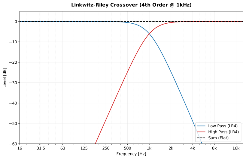

Show the code for this figure

import matplotlib.pyplot as plt
import numpy as np
from scipy.signal import freqz
from phonometry import filters

# Measure both branches: split a unit impulse and take the spectra.
fs = 48000
impulse = np.zeros(fs)
impulse[0] = 1.0
low, high = filters.linkwitz_riley(impulse, fs, freq=1000, order=4)

w, h_lp = freqz(low, worN=8192, fs=fs)
_, h_hp = freqz(high, worN=8192, fs=fs)

fig, ax = plt.subplots(figsize=(9, 5))
ax.semilogx(w, 20 * np.log10(np.abs(h_lp) + 1e-9), label="Low-pass (LR4)")
ax.semilogx(w, 20 * np.log10(np.abs(h_hp) + 1e-9), label="High-pass (LR4)")
ax.semilogx(w, 20 * np.log10(np.abs(h_lp + h_hp) + 1e-9), "--",
            label="Sum (flat)")
ax.set(xlim=(20, 20000), ylim=(-60, 5),
       xlabel="Frequency [Hz]", ylabel="Magnitude [dB]")
ax.grid(True, which="both", alpha=0.3)
ax.legend()
plt.show()

In a real crossover the two branches sum acoustically, not electrically, and the flatness above only survives if the two acoustic paths are time-aligned. A woofer/tweeter acoustic-centre offset of a few centimetres is enough phase rotation at 1 kHz to notch the summation, and the remedy is a delay on the forward driver, not a different filter order. Verify by measuring the summed on-axis response with the swept-sine method of System measurement.

What this guide covers

• Covered

  The five architectures every IEC-band bank can be built on (Butterworth, Chebyshev I/II, Elliptic, Bessel): their magnitude responses compared at the −3 dB crossover and in the full 1/1 and 1/3 octave gallery, the band-edge convention (exact for Butterworth, Chebyshev II and Bessel; the ripple edge for the two equiripple families), and a usage example per architecture, plus the Linkwitz-Riley crossover, whose two branches recombine flat — by sum or by difference, depending on the parity of order/2.

• Not covered

  The band mathematics, the pole-zero, stability and multirate design and the octave_filter() / OctaveFilterBank parameter reference stay in Filter Banks. The IEC 61260-1 Table 1 class acceptance masks, which decide the class each of these architectures actually reaches, are Filter Class Verification.

See also

• Filter Banks: the band mathematics, the design machinery and the parameter reference behind every bank shown here.
• Filter Class Verification (IEC 61260-1): the Table 1 acceptance mask, class 0 and the compliance fiche of these architectures.
• API reference: phonometry and filters.core.
• Theory: Magnitude Responses: what a magnitude response is as a complex transfer function, and how the five architectures differ before any band is filtered.

Quick answers

Which filter architecture should I choose?

Butterworth is the standard choice for general acoustic measurement: a maximally flat passband with no ripple. Chebyshev I gives a sharper roll-off at the cost of passband ripple; Chebyshev II keeps the passband flat and puts the ripple in the stopband instead; Elliptic offers maximum selectivity, with ripple in both bands; and Bessel preserves transient waveform shapes thanks to its linear phase response, but has the slowest roll-off. Note that Chebyshev I and Elliptic take the band edges as their ripple edge rather than their −3 dB point, so their band levels sit a few tenths of a decibel above the other three and must not be mixed with them in one spectrum. Linkwitz-Riley is not one of the five: it is a crossover, and its two branches recombine flat by low + high when order/2 is even and by low - high when it is odd.

References

• American National Standards Institute. (2004). Specification for octave-band and fractional-octave-band analog and digital filters (ANSI S1.11-2004). Acoustical Society of America. The band-edge convention on which every architecture of this gallery places its −3 dB points, which is what makes their band levels comparable.
• International Electrotechnical Commission. (2014). Electroacoustics — Octave-band and fractional-octave-band filters — Part 1: Specifications (IEC 61260-1:2014). The base-10 mid frequencies and band edges that every bank compared in this gallery is designed to, whichever architecture realizes the band.
• Smith, J. O. (n.d.). Introduction to digital filters with audio applications. Center for Computer Research in Music and Acoustics (CCRMA), Stanford University. A free online-book companion treatment of digital-filter design and analysis, covering the classical architectures compared in this gallery.