Data qualification: stationarity and peaks

Every average in this documentation - a PSD, a Leq, a GUM budget - assumes the record is stationary: that the process generating it did not drift while it was being measured. Bendat & Piersol devote Section 10.3 of Random Data to qualifying records before analysis, and phonometry.metrology implements its quantitative core: distribution-free trend and stationarity tests with the book’s own acceptance regions, and the Rice statistics - level crossings, apparent frequency, peak rates and heights - that summarize what a qualified Gaussian record looks like and flag one that is not.

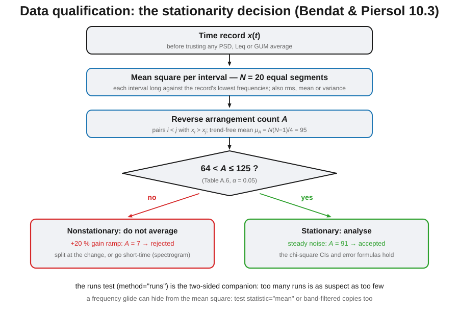
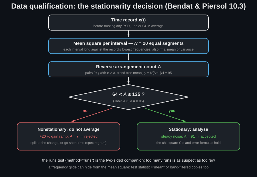
Qualification is a decision, not a statistic, so it reads best as a flow: segment the record, count reverse arrangements, and let the Table A.6 region say whether averaging is allowed.

0. Before the tests: validating the record

Bendat & Piersol’s Section 10.3 covers three activities and this module implements one of them. Qualification — the tests below — asks whether a record is stationary. Validation asks whether it is a record of the thing at all, and it comes first, because every defect in the list below either fails the stationarity test for the wrong reason or, worse, passes it. Validation stays manual, as the book describes it, but it is six lines of numpy and a decision each:

import numpy as np

rng = np.random.default_rng(0)
x = 0.15 * rng.standard_normal(1 << 16)   # your record, in digital units

full_scale = 1.0                          # 1.0 for float audio, 32768 for int16
clipped = int(np.count_nonzero(np.abs(x) >= 0.999 * full_scale))
dead = int(np.max(np.diff(np.flatnonzero(np.diff(x) != 0.0), prepend=0)))
offset = float(np.mean(x) / np.std(x))
spikes = int(np.count_nonzero(np.abs(x - np.mean(x)) > 5 * np.std(x)))
kurtosis = float(np.mean((x - np.mean(x)) ** 4) / np.std(x) ** 4)
print(clipped, dead, round(offset, 4), spikes, round(kurtosis, 2))

Defect	The check	The decision
Clipping	samples at or above 0.999 of full scale	more than a handful and the record is edited or rejected: clipping deflates the high-level crossings of section 4 and inflates every mean square
Dropouts, dead channel	the longest run of identical consecutive samples	any run longer than a few milliseconds is a transmission fault, not a signal
DC offset, infrasonic drift	the record mean against its standard deviation, and the sub-20 Hz share of the PSD against the band of interest	remove the mean and high-pass before section 4, whose formulas assume a zero-mean process
Spikes, transient contamination	samples beyond 5σ, or a kurtosis far above 3 on a supposedly Gaussian record	edit them out and say so, or qualify the record in pieces
Mains hum	peaks at 50 or 60 Hz and their harmonics in a Welch PSD	a fault in the chain, not in the source; fix the grounding rather than the data

The synthetic record above prints 0 1 0.0024 0 3.02, which is what clean looks like: no clipped samples, no repeated sample, an offset of 0.002σ, not one excursion beyond 5σ in 65 536 Gaussian samples, and a kurtosis of 3.0 as a Gaussian record must have.

Alongside the numbers, the acquisition metadata has to travel with the file or none of this is reconstructible later: sample rate, bit depth, gain setting, the calibration factor and the take it came from, microphone and windscreen, and — outdoors — wind speed and temperature. The rule is simply that validation precedes qualification: edit or reject first, then test for stationarity.

1. The reverse arrangement test

Given a sequence of $N$ observations $x_1,\dots ,x_N$ - parameter estimates, segment levels, anything - count the pairs $i<j$ with $x_i>x_j$. Each such pair is a reverse arrangement, and for independent observations of one random variable their total $A$ has (B&P Eqs. (4.54)-(4.55))

$${\mu }_A=\frac{N(N-1)}{4},{\sigma }_A^2=\frac{N(2N+5)(N-1)}{72},$$

with no assumption about the distribution of the $x_i$. A monotonic trend pushes $A$ to an extreme (0 for a rising sequence, $N(N-1)/2$ for a falling one), so the hypothesis of no trend is accepted at significance $\alpha$ when $A$ falls inside a two-sided region - B&P Table A.6, whose $\alpha =0.05$ rows trend_test reproduces exactly and the conformance suite pins. The book’s Example 4.4 (twenty observations, $A=86$, accepted in $(64,125]$) runs verbatim:

from phonometry import trend_test

values = [5.2, 6.2, 3.7, 6.4, 3.9, 4.0, 3.9, 5.3, 4.0, 4.6,
          5.9, 6.5, 4.3, 5.7, 3.1, 5.6, 5.2, 3.9, 6.2, 5.0]

res = trend_test(values)                  # B&P Example 4.4
print(res.statistic, res.bounds)          # 86, (64, 125] — half-open
print(res.trend_free, round(res.p_value, 3))   # True, 0.586
res.plot()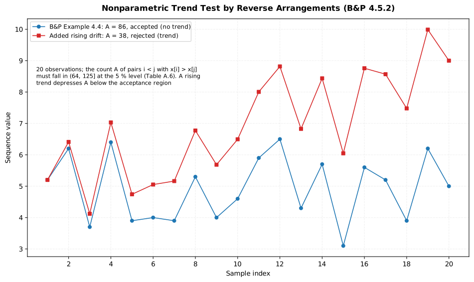

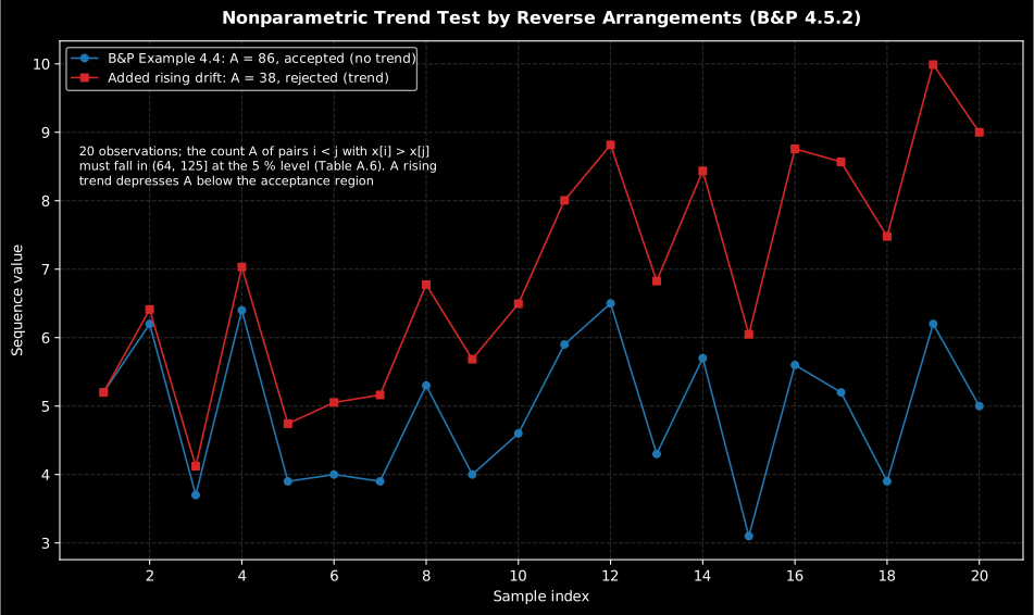
The test never looks at the fitted slope, only at the order of the values. On the left, Bendat & Piersol’s own Example 4.4: $A=86$, comfortably inside the $(64,125]$ acceptance region, $p=0.586$. On the right, the same twenty fluctuations with a drift added that carries them from 5.2 to 9.0: the fluctuations are unchanged, but the ordering is not, and $A$ falls to 38, below the lower bound, at $p=0.0001$. A monotonic drift is what pushes $A$ towards zero, which is why the counting works without knowing the distribution.

Show the code for this figure

import matplotlib.pyplot as plt
import numpy as np
from phonometry import trend_test

example = np.array([5.2, 6.2, 3.7, 6.4, 3.9, 4.0, 3.9, 5.3, 4.0, 4.6,
                    5.9, 6.5, 4.3, 5.7, 3.1, 5.6, 5.2, 3.9, 6.2, 5.0])
drifting = example + np.linspace(0.0, 4.0, example.size)   # rising drift

res_flat = trend_test(example)
res_drift = trend_test(drifting)

fig, ax = plt.subplots(figsize=(10, 6))
index = np.arange(1, example.size + 1)
ax.plot(index, res_flat.values, "o-",
        label=f"Example 4.4: A = {res_flat.statistic}, accepted")
ax.plot(index, res_drift.values, "s-",
        label=f"Rising drift: A = {res_drift.statistic}, rejected")
ax.set_xlabel("Sample index")
ax.set_ylabel("Sequence value")
ax.legend()
plt.show()

bounds is half-open: the hypothesis of no trend is accepted when lower < A <= upper, so $A=125$ passes and $A=64$ does not. The runs test of section 3 uses the same convention, and so does the stationarity verdict of section 2.

The p-value comes from the exact null distribution of $A$ (the inversion counts of a random permutation), computed up to $N=100$ - the range of Table A.6 - and from the book’s normal approximation beyond; the verdict follows the book’s tabulated region. .plot() draws the tested sequence against its sample index with the count, the acceptance region and the verdict in the legend (for method="runs" it also marks the sequence median that classifies each value).

How to read the verdict. It is a hypothesis test, not a measurement. trend_free = True means the data give no evidence of a trend at the chosen level, which is a much weaker statement than “the record is stationary”; $p=0.586$ says the observed count is entirely ordinary for a trend-free sequence, and a $p$ just above 0.05 says almost nothing either way. The consequence that bites in practice is multiplicity: at $\alpha =0.05$ one stationary record in twenty is rejected by construction, so screening the 31 one-third-octave bands of a perfectly stationary record produces one or two rejections as the expected outcome. A single failing band is therefore not evidence of anything; a run of adjacent failing bands, or a failure of the broadband record, is. alpha= is the knob — tighten it when many bands are screened, loosen it when one record must be qualified conservatively — and the acceptance bounds move with it, because they come from the exact null distribution rather than from a table lookup.

2. Stationarity of a record

The B&P Sec. 10.3.1.1 procedure turns the trend test into a stationarity test for a single time history: divide the record into $N$ equal intervals long enough to be independent, compute a mean square value per interval, and test that sequence. Nothing needs to be known about the record’s bandwidth, averaging distribution or units, and the test works on mean values, rms values or variances just as well (statistic=). A running 20 % gain drift - the book’s Example 10.3 scenario - is caught immediately, while the same noise without the drift passes:

import numpy as np
from phonometry import stationarity_test

fs = 8192.0
n = 1 << 16
noise = np.random.default_rng(42).standard_normal(n)

res = stationarity_test(noise, fs)        # 20 segments, mean squares
print(res.stationary, res.count, res.bounds)   # True, 91, (64, 125)

drifting = noise * np.linspace(1.0, 1.2, n)    # +20 % gain ramp
res = stationarity_test(drifting, fs)
print(res.stationary, res.count)          # False, 7  (upward trend -> low A)
res.plot()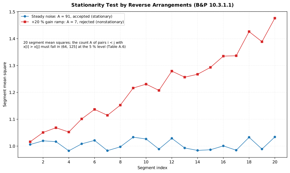

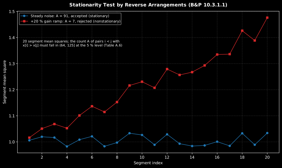
The same twenty-segment sequence tells a stationarity story with the same arithmetic. The steady record’s segment mean squares stay between 0.982 and 1.034 and give $A=91$, inside $(64,125]$. The 20 % gain ramp lifts them from 1.016 to 1.476 — a change of a factor 1.45, which no eye would call dramatic on a time trace — and $A$ collapses to 7. Twenty numbers and a pair counted against a table are enough; nothing about the record’s bandwidth or units enters.

Show the code for this figure

import matplotlib.pyplot as plt
import numpy as np
from phonometry import stationarity_test

fs = 8192.0
n = 1 << 16
steady = np.random.default_rng(42).standard_normal(n)
ramp = np.random.default_rng(42).standard_normal(n) * np.linspace(1.0, 1.2, n)

res_steady = stationarity_test(steady, fs)
res_ramp = stationarity_test(ramp, fs)

fig, ax = plt.subplots(figsize=(10, 6))
index = np.arange(1, res_steady.n_segments + 1)
ax.plot(index, res_steady.segment_values, "o-",
        label=f"Steady noise: A = {res_steady.count}, accepted")
ax.plot(index, res_ramp.segment_values, "s-",
        label=f"+20 % gain ramp: A = {res_ramp.count}, rejected")
ax.set_xlabel("Segment index")
ax.set_ylabel("Segment mean square")
ax.legend()
plt.show()

The result records the per-segment sequence (segment_values, segment_times), the count, the Table A.6 bounds, the exact p_value and the stationary verdict; .plot() draws the sequence with the verdict in the legend. Note that the same reverse-arrangement count answers to two different attribute names in the two result classes, because only one of them has a per-segment sequence to carry:

	trend_test → TrendTestResult	stationarity_test → StationarityTestResult
the count $A$	statistic	count
the verdict	trend_free	stationary
acceptance region	bounds (half-open)	bounds (half-open)
exact p-value	p_value	p_value
the sequence	values	segment_values, segment_times, n_segments

The default of 20 segments matches the book’s worked examples - more segments resolve faster drifts but each interval must stay long against the record’s lowest frequencies for the values to be independent.

How small a drift can it see? Each segment mean square is itself a random variable: for a band of width $B$ observed for $T_{\text{seg}}$ seconds its normalized random error is $1/\sqrt{B{T}_{\text{seg}}}$. Take the default 20 segments over a 10 s record of the 1 kHz one-third-octave band ($B=231$ Hz, $T_{\text{seg}}=0.5$ s): $BT=116$, so each segment value scatters by about 9 %, which is 0.4 dB. A drift much smaller than that cannot be separated from the scatter, while a monotonic drift of a couple of segment standard deviations across the record is rejected almost every time.

Two design consequences follow, and they point in opposite directions to the obvious move. To see a smaller drift, lengthen the record, not the segment count: the scatter falls as $1/\sqrt{T_{\text{seg}}}$ while the trend stays put, so splitting the same record into more segments makes each one noisier. And keep $T_{\text{seg}}$ well above $1/B$ — at least $BT=5$ per interval, and no fewer than ten cycles of the lowest frequency of interest — or the segment values stop being independent and the tabulated acceptance region no longer applies. A 20-segment test of a record band-limited to 20 Hz and above therefore needs intervals of at least 0.5 s, and so a record of at least 10 s.

One shape of nonstationarity escapes this test by construction: a source that alternates between two steady states — a machine that loads and unloads, traffic in platoons — produces a non-monotonic segment sequence that the reverse arrangement test can happily accept while the record is plainly not stationary. That is what method="runs" in section 3 is for, and the honest answer is usually to split the record by state (segment_times shows where) and qualify each part on its own.

Two caveats from the book are worth repeating. A record can be nonstationary with a stationary mean square (a frequency glide, for instance), so pass statistic="mean" or test band-filtered versions when that matters; and the test needs the trend to be slow against the segment length, or it dissolves into the random fluctuation of the segment values.

The first caveat is the one that costs a reader a wrong result, because it makes the test accept a record it should reject. It is worth seeing:

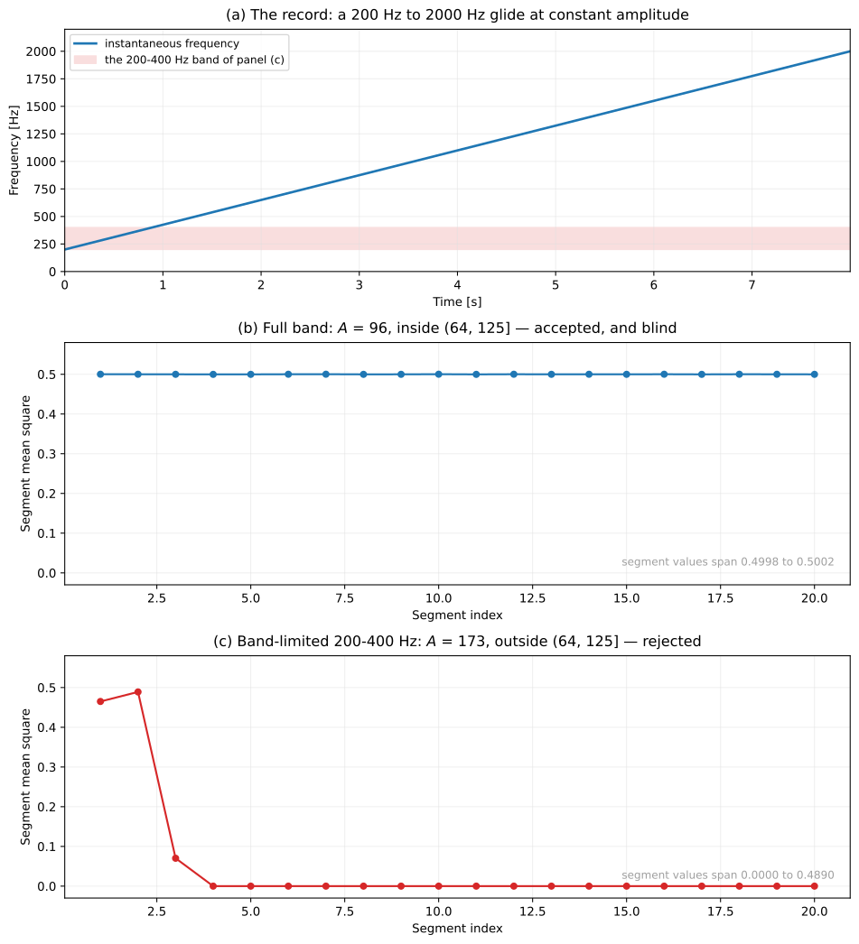
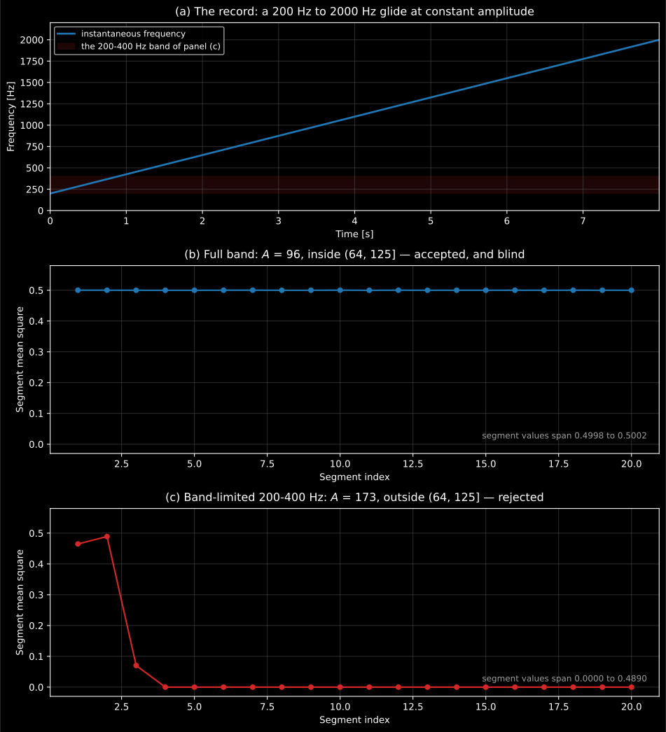
A constant-amplitude glide from 200 Hz to 2 kHz is as nonstationary as a record gets, and the full-band mean square cannot see it: the twenty segment values span 0.4998 to 0.5002 and the count $A=96$ sits comfortably inside $(64,125]$. Band-limit the same record to 200-400 Hz first and the segment values collapse once the glide leaves the band, giving $A=173$ — above the upper bound, and rejected. The remedy in the caveat above is not a formality: what the test sees depends entirely on the statistic and the band you hand it.

Show the code for this figure

import matplotlib.pyplot as plt
import numpy as np
from scipy import signal

# stationarity_test is the one imported in section 2 above.
fs = 8192.0
t = np.arange(1 << 16) / fs
glide = np.sin(2 * np.pi * (200 * t + (2000 - 200) / (2 * t[-1]) * t ** 2))
sos = signal.butter(6, [200 / (fs / 2), 400 / (fs / 2)], btype="band",
                    output="sos")

full = stationarity_test(glide, fs)
banded = stationarity_test(signal.sosfiltfilt(sos, glide), fs)
print(full.count, full.stationary)       # 96 True   -- blind
print(banded.count, banded.stationary)   # 173 False -- caught

fig, (ax1, ax2) = plt.subplots(2, 1, figsize=(10, 7))
for ax, res, label in ((ax1, full, "full band"),
                       (ax2, banded, "200-400 Hz")):
    ax.plot(np.arange(1, res.n_segments + 1), res.segment_values, "o-")
    ax.set_ylim(-0.03, 0.58)
    ax.set_title(f"{label}: A = {res.count}, accept {res.bounds}")
    ax.set_xlabel("Segment index")
    ax.set_ylabel("Segment mean square")
plt.show()

3. The runs test

The classical companion (tabulated in the third edition of Random Data; the exact distribution is Wald & Wolfowitz 1940) classifies each value as above or below the sequence median and counts runs of like classification. A trend or slow drift produces few long runs; rapid alternation produces too many. method="runs" applies it with the exact conditional distribution at any $N$ - for twenty values split 10/10 the acceptance region at $\alpha =0.05$ is the classical $(6,15]$:

import numpy as np
from phonometry import trend_test

rng = np.random.default_rng(3)
res = trend_test(rng.standard_normal(40), method="runs")
print(res.statistic, res.bounds, res.trend_free)
res.plot()   # the sequence about its median with the runs verdict

alternating = np.tile([1.0, -1.0], 10)   # 20 runs: rejected the other way
print(trend_test(alternating, method="runs").trend_free)   # False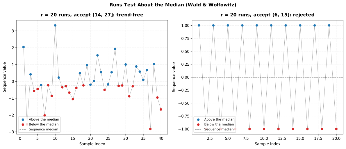

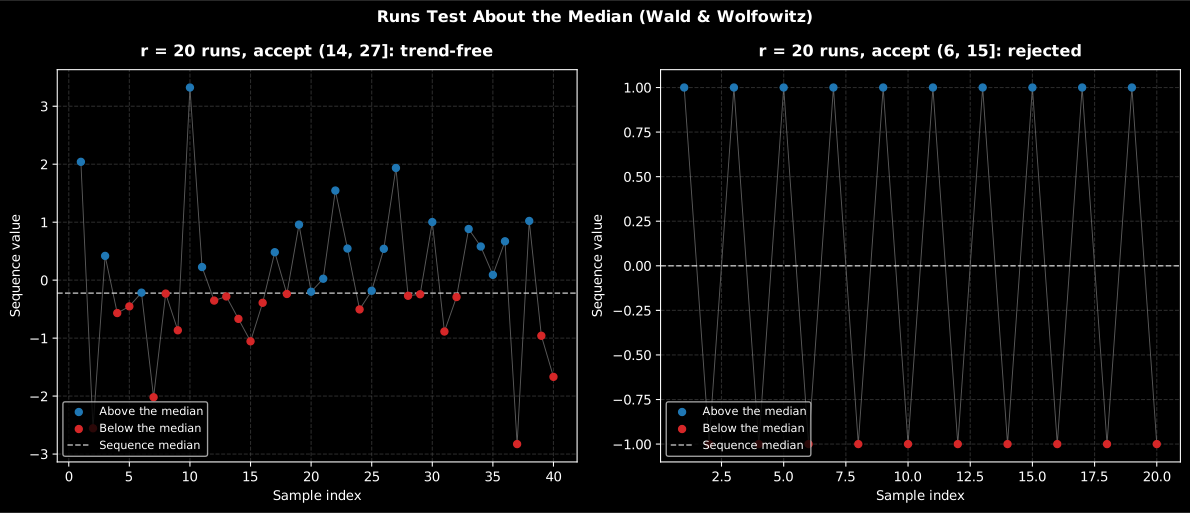
The two-sided verdict of the runs test: 20 runs is unremarkable for 40 Gaussian observations (left, accepted), but the same count from a strictly alternating 20-value sequence exceeds its upper bound (right, rejected): too many runs is as non-random as too few.

Show the code for this figure

import matplotlib.pyplot as plt
import numpy as np
from phonometry import trend_test

rng = np.random.default_rng(3)
sequences = [rng.standard_normal(40), np.tile([1.0, -1.0], 10)]

# One line per sequence — the tested values with the verdict:
trend_test(sequences[0], method="runs").plot()
plt.show()

# Both verdicts side by side, classified about the median:
fig, axes = plt.subplots(1, 2, figsize=(11, 4.5))
for ax, seq in zip(axes, sequences):
    res = trend_test(seq, method="runs")
    idx = np.arange(1, seq.size + 1)
    median = np.median(seq)
    above = seq > median
    ax.plot(idx, seq, "0.7", lw=0.7)
    ax.scatter(idx[above], seq[above], label="above the median")
    ax.scatter(idx[~above], seq[~above], color="r",
               label="below the median")
    ax.axhline(median, color="k", linestyle="--")
    lo, hi = res.bounds
    verdict = "trend-free" if res.trend_free else "rejected"
    ax.set_title(f"r = {res.statistic} runs, accept ({lo}, {hi}]: {verdict}")
    ax.set(xlabel="Sample index", ylabel="Sequence value")
    ax.legend()
plt.show()

The reverse arrangement test is the more powerful of the two against the monotonic trends that dominate practice (B&P Sec. 4.5.2), which is why it is the default everywhere; the runs test adds sensitivity to non-monotonic clustering.

4. Level crossings and the apparent frequency

For a zero-mean Gaussian record with one-sided autospectrum $G(f)$, Rice’s classical results give the expected rate of zero crossings (both slopes, B&P Eq. (5.195)) from the plain frequency moments $m_k=\int f^{k}G(f)\mathrm{d}f$:

$$N_0=\frac{1}{\pi }\frac{{\sigma }_v}{{\sigma }_x}=2\sqrt{\frac{m_2}{m_0}},N_a=N_0{e}^{-a^2/2{\sigma }_x^2},$$

where $N_a$ is the crossing rate of level $a$ (Eq. (5.196)). $N_0/2$ is the record’s apparent frequency: a 60 Hz sine crosses zero 120 times per second, low-pass noise of bandwidth $B$ gives $N_0=2B/\sqrt{3}$ (an apparent frequency of $0.58B$, Example 5.12) and a band centred on $f_c$ gives $N_0=2\sqrt{f_c^2+B^2/12}$ (Example 5.13). level_crossing_rate counts the actual crossings of each level and puts the Rice curve next to them, taking the moments from the record’s own Welch autospectrum:

import numpy as np
from phonometry import level_crossing_rate

fs = 8192.0
t = np.arange(1 << 16) / fs
x = np.sin(2 * np.pi * 60.0 * t)          # a 60 Hz sine ...

res = level_crossing_rate(x, fs)
print(round(res.zero_crossing_rate, 1))   # ... has 120 zeros per second
print(round(res.apparent_frequency, 1))   # 60.0
res.plot()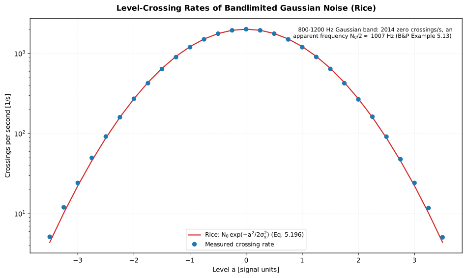

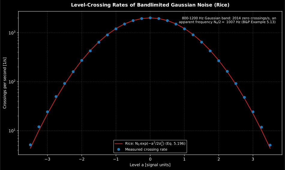
Two moments of the spectrum predict a curve spanning nearly three decades of rate. The measured zero-crossing rate of this 800-1200 Hz record is 2012.7 crossings per second against Example 5.13’s closed form $2\sqrt{f_c^2+B^2/12}=2013.3$, an apparent frequency of 1007 Hz; from there the Rice exponential $N_a=N_0{e}^{-a^2/2{\sigma }_x^2}$ tracks the counts to within 2 % out to $2\sigma$, where the rate has already fallen to 268/s. Past $3\sigma$ the count is a handful of events per second and the scatter is the statistics of the record, not a failure of the model.

Show the code for this figure

import matplotlib.pyplot as plt
import numpy as np
from phonometry import level_crossing_rate

fs = 20480.0
n = 1 << 19
rng = np.random.default_rng(0)
freqs = np.fft.rfftfreq(n, 1 / fs)        # bandlimited Gaussian noise:
spec = rng.standard_normal(freqs.size) + 1j * rng.standard_normal(freqs.size)
spec[(freqs < 800.0) | (freqs > 1200.0)] = 0.0
x = np.fft.irfft(spec, n)

res = level_crossing_rate(x, fs, levels=np.linspace(-3.5, 3.5, 29) * np.std(x))

fig, ax = plt.subplots(figsize=(10, 6))
ax.plot(res.levels, res.rice_rates, label="Rice (Eq. 5.196)")
ax.plot(res.levels, res.rates, "o", label="Measured")
ax.set_yscale("log")
ax.set_xlabel("Level a [signal units]")
ax.set_ylabel("Crossings per second [1/s]")
ax.legend()
plt.show()

The Rice curve holds for Gaussian records, and that is precisely its second use: measured rates that fall systematically off the curve are a quick non-Gaussianity screen (B&P Sec. 5.5.1.1) - clipping shows up as missing high-level crossings, impulsive contamination as an excess. Count-based rates need the record comfortably oversampled: a crossing between two samples of the same sign goes uncounted.

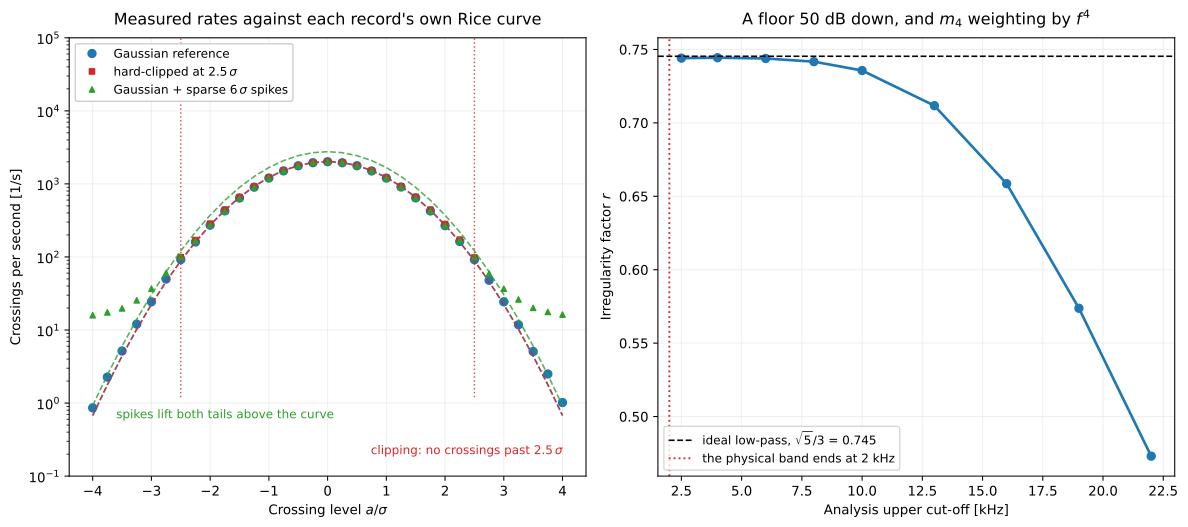
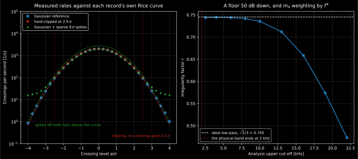
Left: what the screen actually looks like. Three records with the same variance and the same 800-1200 Hz band, each drawn with its own Rice curve so the deviation is a model mismatch and not a scaling artefact. The Gaussian reference sits on the curve at every level. Hard clipping at 2.5σ leaves the rates untouched below the clip level and removes them entirely above it — the signature is a cliff, not a slope. Sparse 6σ spikes lift both tails above the curve beyond about 2.5σ while barely moving the centre. Right: the companion warning of section 5, measured. A record that is ideal low-pass noise to 2 kHz plus a flat floor 50 dB down keeps $r$ at its closed-form 0.745 while the analysis band stays near the physical one, and loses it as the band opens: 0.74 at 6 kHz, 0.71 at 13 kHz, 0.47 at 22 kHz. A noise floor you would never notice on a spectrum plot costs a third of the irregularity factor once the analysis band is ten times too wide.

Finally, the low-frequency half of the same argument, which section 4 opened with and never returned to: the Rice formulas are written for a zero-mean process. Subtract the record mean and high-pass away everything below the physically meaningful band before counting — 20 Hz for an audio-band acoustic record, the transducer’s own lower cut-off for a vibration record. Wind and building rumble sit almost entirely in $m_0$ and contribute almost nothing to $m_2$, so they inflate ${\sigma }_x$ while leaving ${\sigma }_v$ alone and bias $N_0$ and every level-crossing rate low; a slow DC drift can suppress the crossings of the low levels altogether, and a record that never returns to zero has no zero crossings at all. The rule is symmetric: band-limit at both ends, the low end for $m_0$ and the high end for $m_4$, and quote the band you used whenever you report an apparent frequency or an irregularity factor, because neither number means anything without it.

5. Peaks: rates, the irregularity factor and heights

The same moments fix the expected rate of local maxima $M=(1/2\pi )({\sigma }_a/{\sigma }_v)=\sqrt{m_4/m_2}$ (Eq. (5.211)) and with it the dimensionless irregularity factor

$$r=\frac{N_0}{2M}=\frac{m_2}{\sqrt{m_0{m}_4}}\in (0,1],$$

the single number that fixes the distribution of peak heights (B&P Sec. 5.5.4). At $r=1$ - narrow bandwidth data, one maximum per zero-crossing cycle - peaks are Rayleigh distributed: $\mathrm{Prob}[\text{peak}>a]=e^{-a^2/2{\sigma }_x^2}$ (Eq. (5.206)), which is the one-in-3000 chance of a peak beyond $4\sigma$ of B&P Example 5.14. As $r\to 0$ ever more ripples ride on each cycle, negative maxima appear, and the peak heights approach the plain Gaussian amplitude distribution. In between, Rice’s mixture (Eqs. (5.217)/(5.223)) interpolates the two, available as peak_exceedance() / peak_density() on the result:

import numpy as np
from phonometry import peak_statistics

fs = 8192.0
t = np.arange(1 << 16) / fs
x = np.sin(2 * np.pi * 60.0 * t)          # narrowband: r is essentially 1

res = peak_statistics(x, fs)
print(round(res.irregularity_factor, 3))       # 0.997
print(res.peak_exceedance(4.0))                # exp(-8): about 1 in 3000
res.plot()   # empirical exceedance against the Rice mixture (figure below)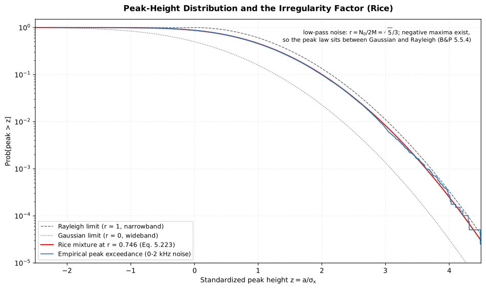

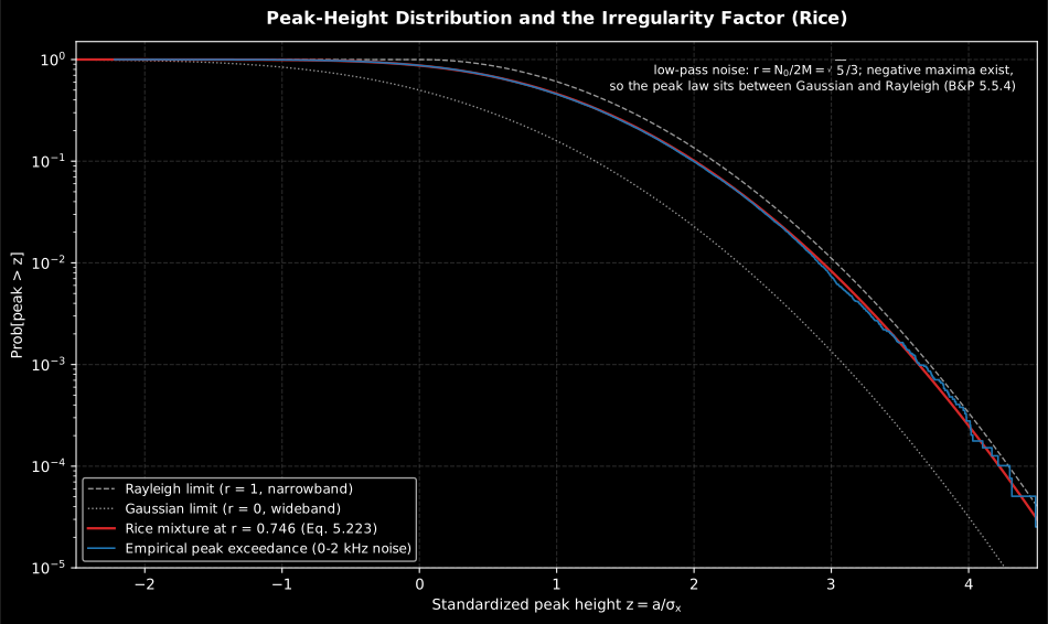
One number decides which curve the peaks follow. Ideal low-pass noise has the closed-form $r=\sqrt{5}/3=0.745$, and the record measures 0.746 — which is also why 12.6 % of its 39 534 maxima are negative, an impossibility under Rayleigh. The empirical staircase sits on the Rice mixture for that $r$ and between the two limits everywhere: the chance of a peak beyond $4\sigma$ is $2.5\times 10^{-4}$, a quarter below the Rayleigh $e^{-8}=3.4\times 10^{-4}$. Assuming the Rayleigh limit on a record that is not narrowband over-predicts the extremes.

Show the code for this figure

import matplotlib.pyplot as plt
import numpy as np
from phonometry import peak_statistics
from phonometry.metrology.data_qualification import _rice_peak_exceedance

fs = 20480.0
n = 1 << 19
rng = np.random.default_rng(3)
freqs = np.fft.rfftfreq(n, 1 / fs)        # low-pass noise: r = sqrt(5)/3
spec = rng.standard_normal(freqs.size) + 1j * rng.standard_normal(freqs.size)
spec[freqs > 2000.0] = 0.0
x = np.fft.irfft(spec, n)

res = peak_statistics(x, fs)
peaks = res.peak_values
empirical = 1.0 - np.arange(1, peaks.size + 1) / peaks.size
z = np.linspace(-2.5, 4.5, 400)

fig, ax = plt.subplots(figsize=(10, 6))
ax.plot(z, _rice_peak_exceedance(z, 1.0), "--", label="Rayleigh (r = 1)")
ax.plot(z, _rice_peak_exceedance(z, 0.0), ":", label="Gaussian (r = 0)")
ax.plot(z, res.peak_exceedance(z),
        label=f"Rice (r = {res.irregularity_factor:.3f})")
ax.plot(peaks, empirical, drawstyle="steps-post", label="Empirical")
ax.set_yscale("log")
ax.set_ylim(1e-5, 1.5)
ax.set_xlabel(r"Standardized peak height $z = a/\sigma_x$")
ax.set_ylabel("Prob[peak > z]")
ax.legend()
plt.show()

For an ideal low-pass band the closed forms give $r=\sqrt{5}/3=0.745$, and the measured value lands on it. The irregularity factor is the standard bridge to fatigue and vibro-acoustic damage estimation, where it selects the cycle-counting correction between the narrow-band Rayleigh assumption and broad-band rainflow corrections. One practical warning: $m_4$ weights the spectrum by $f^4$, so wideband instrumentation noise far above the physical band silently inflates $M$ and deflates $r$ - band-limit the record to the physically meaningful range first.

Where this fits

Qualification comes before the statistics this section’s other pages compute: the chi-square confidence interval of a Welch PSD and the random-error formulas of the correlation estimators all assume the record is stationary, as does the very idea of the $L_{eq}$ of a measurement in Levels. When a record fails the test, split it at the change (the segment_values sequence shows where), analyse the pieces, or move to the short-time views - the calibrated spectrogram - that do not assume stationarity. And when it passes, the GUM machinery can propagate the remaining random error of every averaged estimate with a clean conscience.

What this guide covers

• Covered

  Bendat & Piersol Section 4.5.2 with Table A.6 (the reverse arrangement trend test, trend_test, its exact and normal-approximation p-value and Example 4.4), the Wald & Wolfowitz (1940) runs test (trend_test(method="runs")), the Section 10.3.1.1 segment mean-square stationarity procedure with Example 10.3 (stationarity_test), and the Rice (1945) level-crossing and peak statistics of Section 5.5 (level_crossing_rate, peak_statistics, the irregularity factor and its Rayleigh/Gaussian peak-height limits).

• Not covered

  Section 10.3 of the book is titled “data qualification” more broadly and also covers classification, validation and editing procedures; phonometry.metrology implements only its quantitative core, the segment mean-square stationarity test. Classifying a record’s type, validating it against physical limits, or editing out glitches stay manual steps the way the book describes them, outside this module.

See also

• Spectral analysis: the chi-square confidence interval that assumes the stationarity this page tests.
• Time-frequency analysis: the short-time view for records that fail the test, and for the glides its mean square cannot see.
• GUM uncertainty: propagating the remaining random error of a qualified average.
• Levels: the $L_{eq}$ whose definition assumes one stationary measurement.
• API reference: metrology.data_qualification.
• Theory: Measurement uncertainty (GUM): the uncertainty framework the qualification criteria of this page feed.

References

• Bendat, J. S., & Piersol, A. G. (2010). Random data: Analysis and measurement procedures (4th ed.). Wiley. https://doi.org/10.1002/9781118032428Section 4.5.2 with Table A.6 (the nonparametric reverse arrangement trend test, its mean and variance, the tabulated percentage points and Example 4.4), Section 10.3 (data qualification: classification, validation, editing; the segment mean-square stationarity procedure of 10.3.1.1 and Example 10.3) and Section 5.5 (level crossings and peak values: Eqs. (5.195)-(5.196), (5.206), (5.211), (5.217)-(5.223) and Examples 5.12-5.15). ISBN 978-0-470-24877-5. The runs companion appeared in the third edition's percentage points of the run distribution.
• Rice, S. O. (1945). Mathematical analysis of random noise. The Bell System Technical Journal, 24(1), 46-156. https://doi.org/10.1002/j.1538-7305.1945.tb00453.xThe original derivations of the expected level-crossing and maxima rates and the peak distribution of Gaussian noise that Bendat & Piersol Section 5.5 presents (their Ref. 6; Parts I-II are in volume 23, 1944).
• Wald, A., & Wolfowitz, J. (1940). On a test whether two samples are from the same population. The Annals of Mathematical Statistics, 11(2), 147-162. https://doi.org/10.1214/aoms/1177731909The exact conditional distribution of the number of runs, from which the runs-about-the-median acceptance regions are computed.