Free-Field Corrections of a Sound Level Meter (IEC 62585)
Standards: IEC 62585IEC 61672IEC/TS 61094JCGM 100
A periodic test of a sound level meter by IEC 61672-3 does not put the meter in an anechoic room. It drives the microphone with a sound calibrator, a comparison coupler or an electrostatic actuator, and none of those is the plane progressive wave the meter is specified for: the microphone and the case respond differently to a pressure in a small cavity, or to an electrostatic force on the diaphragm, than to a wave arriving from the front. The test therefore needs, at each frequency, the correction that turns what the meter indicates on that source into what it would indicate in a free field of the same level, and the manufacturer has to state it in the manual. IEC 62585:2012 gives the methods for finding those corrections, the uncertainty they may carry, and the adjustment value the manual quotes at the calibration check frequency.
This page runs every step on a synthetic class 1 meter and on the two worked budgets the standard prints.
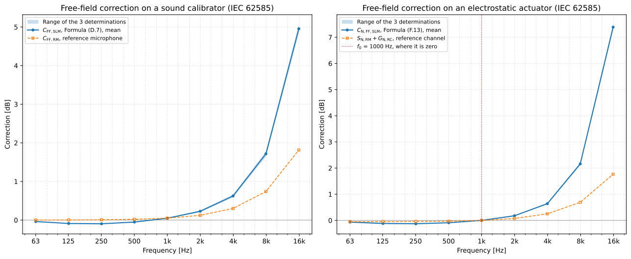
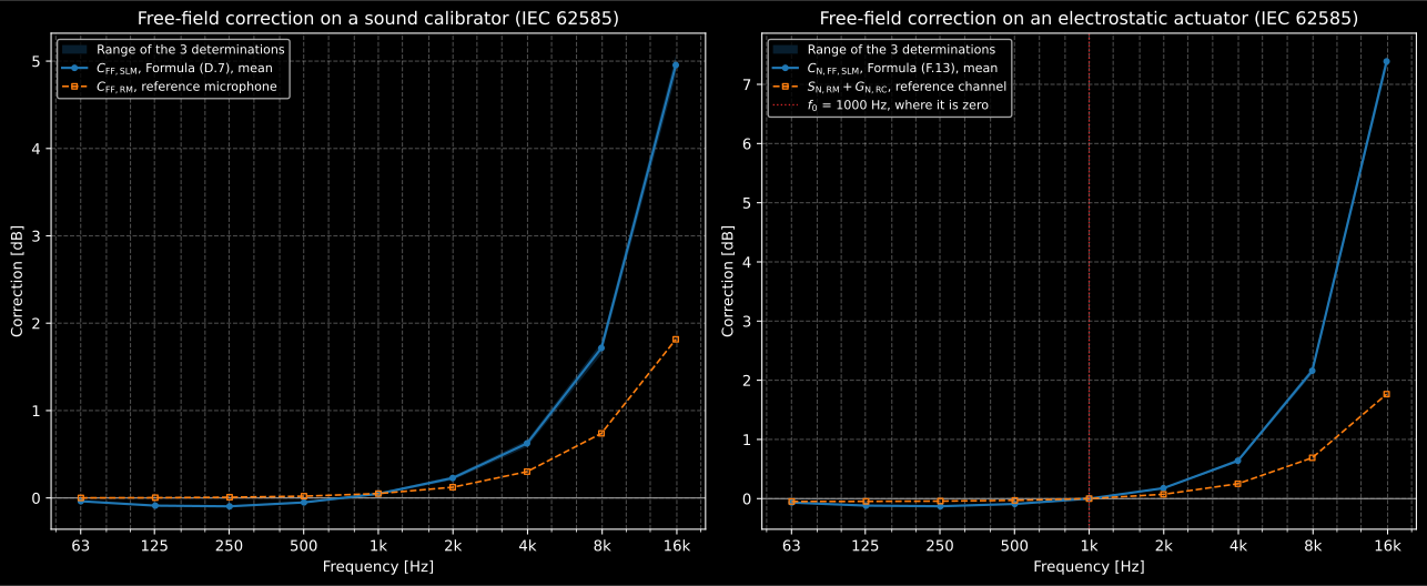
The correction of the synthetic meter on its calibrator (left) and on an
electrostatic actuator (right), from the results’ own .plot().
1. The adjustment value at the calibration check frequency
Section titled “1. The adjustment value at the calibration check frequency”A sound level meter is adjusted in use by applying its calibrator and setting the display. What the display should read is not the level stated for the calibrator, : the manufacturer first sets the sensitivity so that the free-field response of the meter deviates as little as it can from the incident level over the whole frequency range, and only then applies the calibrator and reads . The manual states the adjustment value (Annex A)
as a fixed number, without an uncertainty (clause 8), and it can leave a deliberate offset at the calibration check frequency itself, because the fit is over the whole range (NOTE 1 of clause 8).
The text asks for the sensitivity that minimises “the averaged deviation” and
says the tolerance limits of IEC 61672-1, which vary with frequency, “shall be
taken into account”, but it prints no formula. metrology.adjustment_value
takes the least-squares reading: the adjustment minimises
, being the deviation at frequency and
for a tolerance , so a band with a tight tolerance pulls
the fit harder than one with a loose one:
with what the meter reads on the calibrator at the sensitivity the
free-field readings were taken at. Here the tolerances are the narrower side
of the class 1 acceptance limits of IEC 61672-1 Table 3, which
filters.weighting_class_limits holds:
import numpy as npfrom phonometry import filters, metrology
f3 = metrology.exact_frequencies(63, 16000, fraction=3)   # 25 exact one-third octavesnominal, lower, upper = filters.weighting_class_limits(1)  # IEC 61672-1 Table 3, class 1band = (nominal >= 63) & (nominal <= 16000)tolerance = np.minimum(upper, -lower)[band]                # the narrower side at each band
x3 = f3 / 1000response = 0.4 + 0.12 * np.cos(3 * np.log(x3)) - 0.3 * (x3 / 8) ** 2   # indication less field, dBa = metrology.adjustment_value(    f3,    94.0 + response,           # the meter in a 94 dB free field, before the adjustment    94.35,                     # L4': the same meter on its calibrator    calibrator_level_db=94.0,  # L1, stated for the calibrator    tolerance_db=tolerance,)print(round(a.sensitivity_adjustment_db, 2), round(a.adjustment_db, 2))  # -0.37 0.02print(round(a.check_frequency_offset_db, 2))                           # 0.15a.plot()
The fit lowers the sensitivity by 0,37 dB, the calibrator then reads
93,98 dB, and the manual states dB. At 1 kHz the adjusted
meter reads a free field 0,15 dB high, : that is the offset the
fit chose so that the response sits inside the tolerances everywhere else. A
tolerance of np.inf leaves a band out of the fit, and
pressure_indicated_level_db= adds the pressure response, from which
pressure_to_free_field_correction_db and follow.
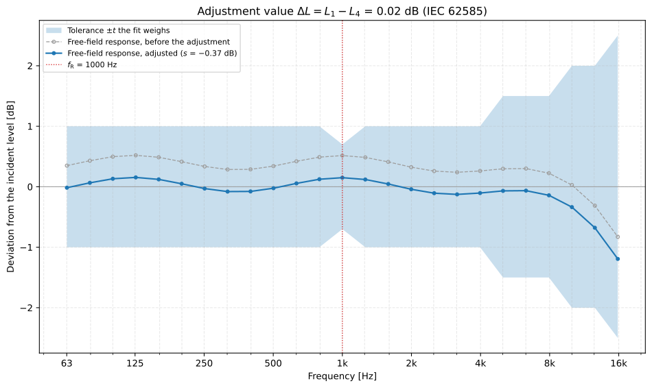
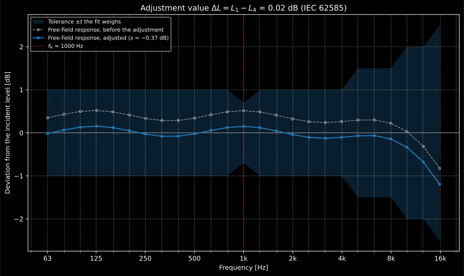
The free-field response before and after the adjustment, inside the class 1 tolerances it was weighed against.
2. How the measurement goes
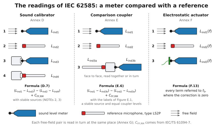
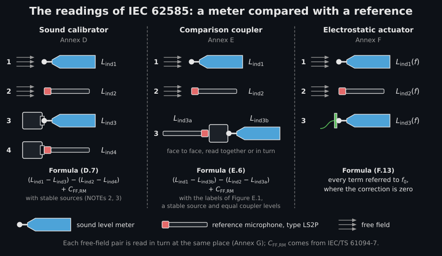
Section titled “2. How the measurement goes”Every method compares the meter with a laboratory standard microphone of type LS2P, whose free-field correction is known from IEC/TS 61094-7, first in a free progressive field and then on the source. The comparison is by substitution (Annex G): the meter is measured, removed, and the reference put in its place, so neither needs an absolute calibration.
| Requirement | Value | Clause |
|---|---|---|
| Environment | 80 kPa to 105 kPa, 20 °C to 26 °C, 25 % to 70 % relative humidity; below 97 kPa an extra component enters the budget | 6 |
| Reference conditions | 23 °C, 101.325 kPa, 50 % relative humidity | 4 |
| Free-field mounting | On a rod of the microphone’s diameter; source more than 1 m away and at least six times the largest dimension of the meter; sound in the reference direction | 6 |
| Meter support | A non-vertical rod at the rear, method 1 or 2 of Figure 1 (method 2 at less than 60°); method 3 is not used | 6 |
| Samples | Three calibrators, three microphones and one meter; five microphones for a typical response, five windscreens | 7 |
| Source level | 70 dB to 125 dB in a calibrator or coupler, preferably the reference level at 1 kHz; 80 dB to 105 dB on the display at 1 kHz with an actuator | 12, 13, 14 |
| Frequencies | Octaves from 63 Hz to 16 kHz (class 1) or 8 kHz (class 2) for a microphone; exact base-ten frequencies of Annex H | 10, B.2, C.2 |
| Determinations | Nine for a calibrator (three microphones on three calibrators), three microphones for a coupler, the combinations of clause 7 for an actuator; the correction is their mean | D.2, E.2, F.2 |
3. The corrections for a calibrator, a coupler and an actuator
Section titled “3. The corrections for a calibrator, a coupler and an actuator”Annex D, a multi-frequency sound calibrator. Four readings (Figure D.1): the meter in a free field, ; the reference in its place, ; the calibrator on the meter, ; the same calibrator on the reference, . The correction is the meter’s free-field response relative to its response on the calibrator, carried over from the reference:
where the two level differences are the drift of the free field between the first two measurements and the difference of the calibrator’s level on the two microphones, both zero for stable sources. Each reading may be a row per determination, and the result keeps every one:
f = metrology.exact_frequencies(63, 16000, fraction=1)   # the nine exact octavesx = f / 1000c_ff_rm = 0.05 * x**1.3                        # C_FF,RM of the reference: illustrativefree = 0.1 * np.sin(np.log(x)) - 0.05 * x**1.2  # the meter in a free field, re the fieldpressure = -0.1 * x**1.5                        # the meter on the calibrator, re its levelspread = np.array([[0.0], [0.02], [-0.03]]) * x**0.8   # three microphones of the model
c = metrology.sound_calibrator_correction(    f,    94.0 + free + spread,          # L_ind1: the meter in the free field    94.0 + c_ff_rm,                # L_ind2: the reference in its place    94.0 + pressure + spread / 2,  # L_ind3: the calibrator on the meter    94.0,                          # L_ind4: the calibrator on the reference    reference_free_field_correction_db=c_ff_rm,)print(c.correction_db.round(2))  # [-0.04 -0.09 -0.1  -0.05  0.05  0.23  0.63  1.72  4.95]print(c.range_db.round(2))       # [0.   0.   0.01 0.01 0.02 0.04 0.08 0.13 0.23]print(c.clause, c.formula)       # 12 D.7c.plot()
The values of c_ff_rm here only stand in for the free-field correction of a
real reference microphone; take yours from IEC/TS 61094-7 or from the
microphone’s calibration. The correction climbs above 2 kHz because the
calibrator presses on the diaphragm while a free field also diffracts round
the microphone and the case.
The three rows here are three microphones on one calibrator. D.2 step 6 asks
for nine determinations, three microphones on three calibrators, and clause 12
judges “the range of correction values at each frequency measured using a
sample of three microphones”, not the spread between the calibrators. Given
nine rows, microphones=[1, 1, 1, 2, 2, 2, 3, 3, 3] says which rows share a
microphone, and range_db is then the range of the three microphones’ mean
corrections, microphone_corrections_db. Without it every row counts as a
microphone of its own, as the three rows above do.
Annex E, a comparison coupler. The meter and the reference face each other
in the two openings of one cavity, so the third measurement reads both at
once. metrology.comparison_coupler_correction takes the same free-field
readings and the two readings in the coupler, slm_coupler_level_db and
reference_coupler_level_db, named by what each is of. That naming is on
purpose: Figure E.1, its list of symbols and Table I.1 call the reference’s
reading and the meter’s , while Formulas
(E.4) to (E.6) are written the other way round, as (D.5) to (D.7) are for a
calibrator. Read with the figure’s labels, the printed (E.6) comes out
away from the
correction, the deviations of the two channels’ indications from the level in
the coupler. The reference channel reads the output voltage of its microphone
and the method needs no absolute calibration (E.1, E.2), so that difference
carries the two channels’ absolute sensitivities and is there at every
frequency; only when both channels read sound pressure level does it shrink to
twice the difference of the two pressure responses. The defect is in the
errata register.
Annex F, an electrostatic actuator. An actuator is not an absolute source, so its correction is normalised to the calibration check frequency , where it is zero, and the absolute response there comes from a sound calibrator (NOTE 2 of F.2). Every term is referred to , , and the reference contributes its free-field sensitivity and the gain of its channel :
e = metrology.electrostatic_actuator_correction( f, 94.0 + free + spread, # L_ind1(f) 94.0 - 26.0 + c_ff_rm, # L_ind2(f): the reference channel, dB re 1 V 94.0 - 0.08 * x**1.7 + spread / 2, # L_ind3(f): the actuator on the meter reference_sensitivity_level_db=-26.0 + c_ff_rm, # S_RM(f), dB re 1 V/Pa)print(e.correction_db.round(2)) # [-0.07 -0.12 -0.13 -0.09 0. 0.18 0.64 2.16 7.39]The drive voltage of the actuator is taken to be independent of frequency, so
its simulated level is the same at and (NOTE 4); pass
actuator_level_db= when it is not, and reference_channel_gain_db= for a
reference channel that is not flat.
4. The uncertainty budget of Annex I
Section titled “4. The uncertainty budget of Annex I”Table I.1 lists fifteen likely components of the uncertainty of a correction
measured with a comparison coupler, each with the distribution that sets its
divisor: the half-width of a rectangular distribution over for most,
the expanded uncertainty of from IEC/TS 61094-7 over 2, and
the repeatability from repeat measurements over 1, with its degrees of freedom.
Tables I.2 and I.3 fill it in at 1 kHz and 8 kHz.
metrology.correction_uncertainty_budget builds the budget on
metrology.combine_uncertainty, every component a correction entering
Formula (E.6) with a sensitivity of , and takes the coverage factor
from the Welch-Satterthwaite effective degrees of freedom at a level of
confidence of 95 % (clause 5):
table_i2 = {    "a1": 0.005, "a2": 0.005, "a3": 0.005, "a4": 0.005,   # the four level readings    "a5": 0.05, "a6": 0.0,                                  # the two level differences    "a7": 0.06,                                             # U of C_FF,RM (k = 2)    "a8": 0.025, "a9": 0.025, "a10": 0.029,                 # gains and distance    "a11": 0.013, "a12": 0.013, "a13": 0.0, "a14": 0.005,   # field, mountings, diameters, rounding    "a15": 0.03,                                            # repeatability (k = 1)}b1 = metrology.correction_uncertainty_budget(table_i2, repeatability_dof=2, frequency_hz=1000)print(round(b1.combined_uncertainty_db, 4), round(b1.effective_dof, 2))   # 0.059 29.98print(round(b1.coverage_factor, 2), round(b1.expanded_uncertainty_db, 2))  # 2.04 0.12
table_i3 = {**table_i2, "a7": 0.17, "a11": 0.104, "a12": 0.104, "a15": 0.06}b8 = metrology.correction_uncertainty_budget(table_i3, repeatability_dof=2, frequency_hz=8000)print(round(b8.combined_uncertainty_db, 3), round(b8.coverage_factor, 2),      round(b8.expanded_uncertainty_db, 2))                                # 0.14 2.0 0.28
Both tables reproduce: 0,0590 dB and 29,98 degrees of freedom at 1 kHz,
0,140 dB, and 0,28 dB at 8 kHz. Table I.2 prints , though,
and that is not the factor its own 29,98 degrees of freedom give. At 95 % the
Student factor for 29,98 is 2,042; 2,11 is the one for about 17. The expanded
uncertainty the page’s numbers give is
dB, printed 0,12 either way, but the table’s guard digit, 0,12(4), is the
misprinted at work; the case is in the errata
register. Below 97 kPa,
static_pressure_kpa= adds the component of clause 6 (0,15 dB up to 3 kHz,
0,25 dB above, ), and additional_components= takes any component a
laboratory’s own method needs, such as the drive of an actuator.
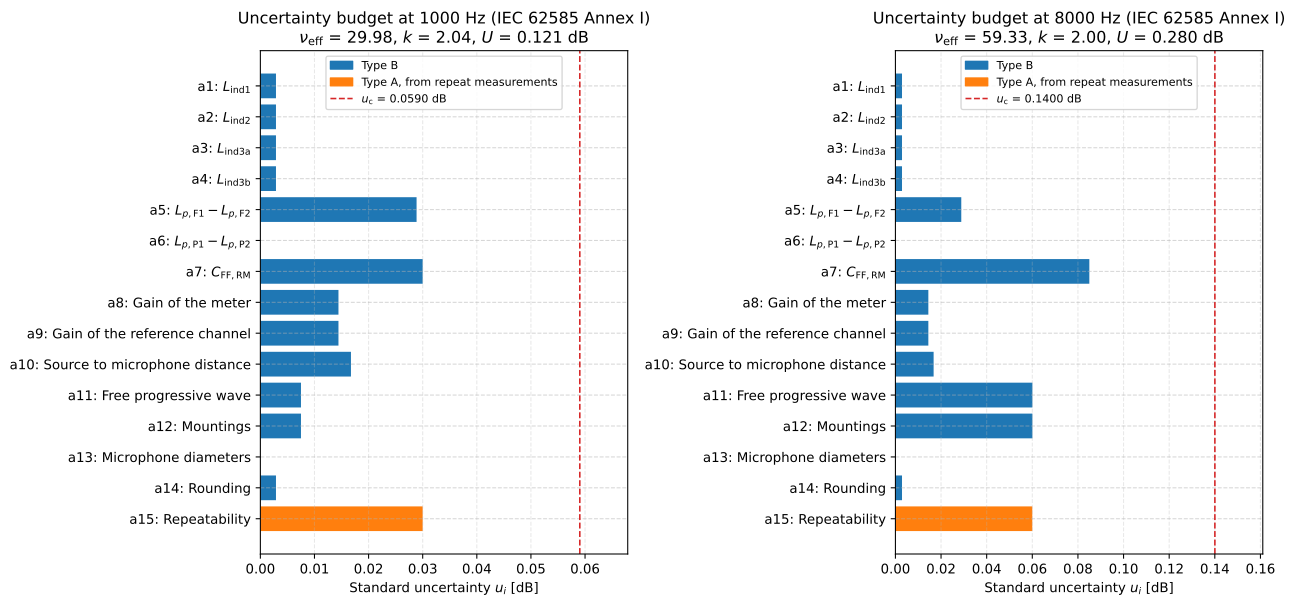
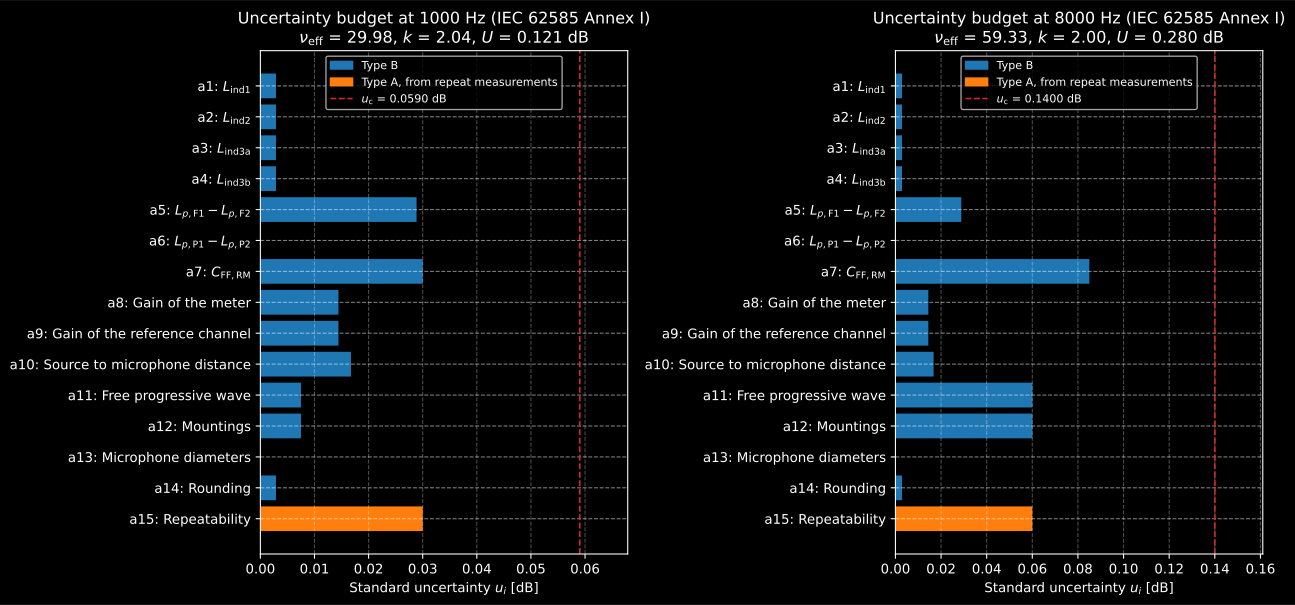
The budgets of Tables I.2 and I.3, one bar per component, the statistical one apart.
5. The maximum permitted uncertainty, and the verdict
Section titled “5. The maximum permitted uncertainty, and the verdict”Each clause states the largest expanded uncertainty a correction may carry and still be used for the manual (clause 5); a measurement that exceeds one is not used. The range is inclusive: “shall not exceed” lets a value equal to its maximum pass, and one that reaches it through floating-point arithmetic too, by the same rule as the IEC TC 29 conformance verdict.
| Clause | Correction for | Maximum expanded uncertainty |
|---|---|---|
| 9 | Reflections from the case, diffraction round the microphone | 0,25 dB up to and including 4 kHz; 0,35 dB above |
| 10 | The microphone’s deviation from a uniform response | 0,25 dB from 63 Hz to 4 kHz; 0,35 dB to 8 kHz; 0,45 dB above |
| 11 | Windscreens and similar accessories | 0,20 dB up to and including 4 kHz; 0,30 dB above |
| 12, 13, 14 | A calibrator, a coupler, an actuator | 0,25 dB up to and including 4 kHz; 0,35 dB below 10 kHz; 0,50 dB from 10 kHz |
Clauses 10 and 11 exclude the variability of the samples of microphone or
accessory. For a calibrator, a coupler or an actuator, clauses 12 to 14 add a
second requirement on the microphone: if the range of the corrections measured
with three microphones exceeds the maximum at a frequency, the microphone is
unsuitable for that source unless more samples show otherwise.
metrology.verify_correction_uncertainty judges both, and a frequency within
2 % of a boundary reads as it, so the exact 3 981 Hz of the 4 kHz band is “up
to and including 4 kHz”. Here each octave of the calibrator’s correction gets a
budget like Table I.2 below 1 kHz, with a reference, a field and a
repeatability that grow above it:
print(metrology.maximum_expanded_uncertainty(f, clause=c.clause))# [0.25 0.25 0.25 0.25 0.25 0.25 0.25 0.35 0.5 ]
a7 = [0.06, 0.06, 0.06, 0.06, 0.06, 0.08, 0.10, 0.17, 0.30]     # U of C_FF,RM, k = 2a11 = [0.013, 0.013, 0.013, 0.013, 0.013, 0.03, 0.06, 0.104, 0.18]  # field and mountingsa15 = [0.03, 0.03, 0.03, 0.03, 0.03, 0.04, 0.05, 0.06, 0.09]    # repeatabilitybudgets = [    metrology.correction_uncertainty_budget(        {**table_i2, "a7": u7, "a11": u11, "a12": u11, "a15": u15},        repeatability_dof=2,        frequency_hz=fx,        correction_db=cx,    )    for fx, u7, u11, u15, cx in zip(f, a7, a11, a15, c.correction_db, strict=True)]v = metrology.verify_correction_uncertainty(    f,    [b.expanded_uncertainty_db for b in budgets],    clause=c.clause,    correction_db=c.correction_db,    coverage_factor=[b.coverage_factor for b in budgets],    correction_range_db=c.range_db,)print(v.passes)              # Trueprint(v.margin_db.round(2))  # [0.13 0.13 0.13 0.13 0.13 0.1  0.06 0.07 0.04]v.plot()v.report("free-field-corrections.pdf")
The verdict is the object, not a boolean: v.passes is the answer,
failing_frequencies_hz says where it fails, and bool(v) raises rather than
let if verify_correction_uncertainty(...): pass every measurement. The
tightest margin is at 16 kHz, 0,04 dB under the 0,50 dB of clause 12.
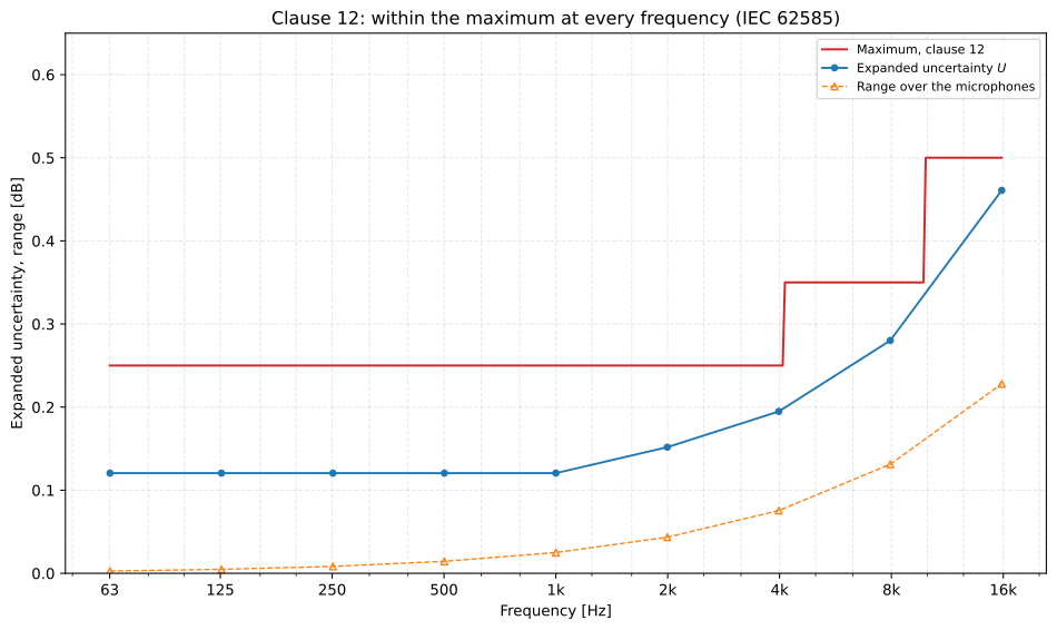
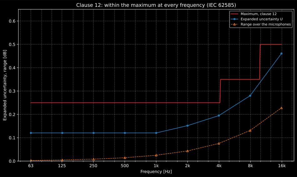
The expanded uncertainty and the range over the microphones, under the maximum of clause 12.
.report() renders what clause 15 n) and o) ask the laboratory to issue: the
corrections with their expanded uncertainties and coverage factors, and a
statement of whether the uncertainties are within the maximum permitted
values. The example fiche is regenerated with make reports and kept rendered
in the repository; click the preview to open the PDF.
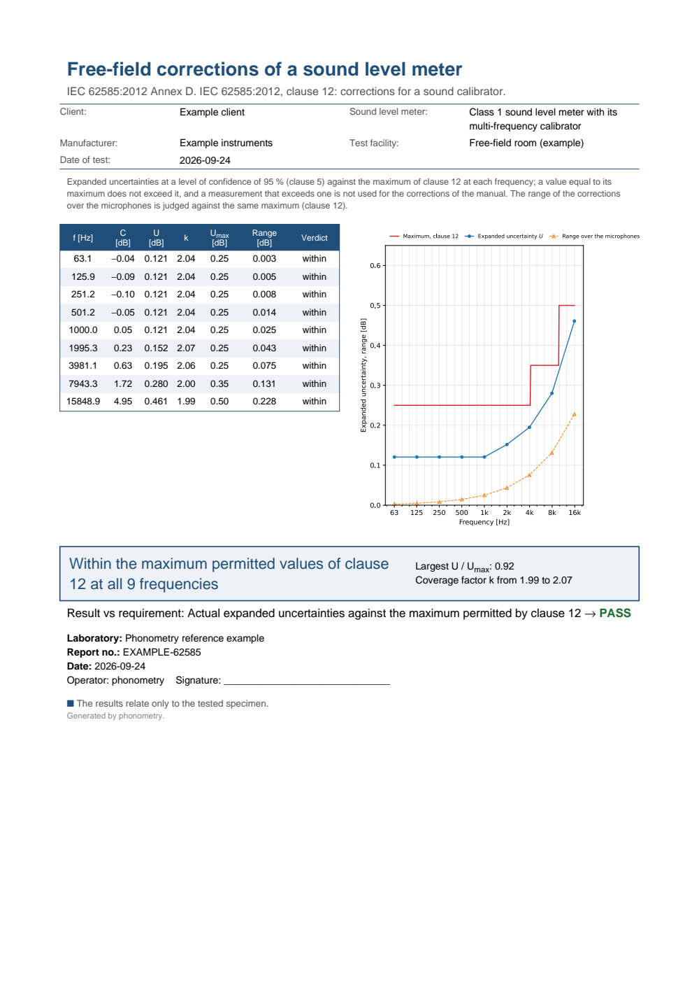
One-page fiche for the corrections of a class 1 sound level meter on its multi-frequency calibrator: a metadata header, the basis line citing IEC 62585:2012 clause 12, a table of the nine exact octaves from 63.1 Hz to 15 848.9 Hz with the correction, the expanded uncertainty, the coverage factor, the maximum, the range over three microphones and the verdict at each, the verification plot beside it, the boxed statement Within the maximum permitted values of clause 12 at all 9 frequencies with the largest U / Umax of 0.92, and a PASS verdict.
6. Exact frequencies
Section titled “6. Exact frequencies”The corrections are measured and reported at exact base-ten frequencies, not at the nominal ones (clause 10, B.2, C.2). Annex H gives them by Formula (H.1),
for every integer , with for one-twelfth-octave steps; Table H.1
prints the decade from 1 kHz to 10 kHz to seven significant digits.
metrology.exact_frequencies evaluates it for any designator, and the octaves
and thirds above came from it:
h = metrology.exact_frequencies(1000, 10000) # the 41 rows of Table H.1print(h.size, (h[[1, 31, 40]] / 1000).round(6)) # 41 [ 1.059254 5.956621 10. ]All 41 values reproduce. The exponent column prints for index 31, where its own value is ; the library evaluates the formula and never reads that column.
Show the code for these figures
import matplotlib.pyplot as plt
fig, (ax_calibrator, ax_actuator) = plt.subplots(1, 2, figsize=(13.5, 5.6))c.plot(ax_calibrator)e.plot(ax_actuator)fig.tight_layout()
fig, ax = plt.subplots(figsize=(10, 6))a.plot(ax)fig.tight_layout()
fig, (ax_1k, ax_8k) = plt.subplots(1, 2, figsize=(13.5, 6.4))b1.plot(ax_1k)b8.plot(ax_8k)fig.tight_layout()
fig, ax = plt.subplots(figsize=(10, 6))v.plot(ax)fig.tight_layout()plt.show()
What this guide covers
Section titled “What this guide covers”Covered
IEC 62585:2012, the calculations of Annexes A, D, E, F, H and I: the adjustment value of Annex A, with the pressure-to-free-field correction and the levels to of Figure A.1; the free-field corrections for a multi-frequency sound calibrator (Formula (D.7)), a comparison coupler (Formula (E.6), with the readings named by what they are of) and an electrostatic actuator (Formula (F.13), normalised to the calibration check frequency), averaged over the determinations with their range over the microphones kept; the uncertainty budget of Annex I with the fifteen components of Table I.1, the static-pressure component of clause 6 and the Welch-Satterthwaite coverage factor; the maxima of clauses 9 to 14 and the range requirement of clauses 12 to 14 as a verdict and a fiche; and the exact frequencies of Annex H. Tables I.2, I.3 and H.1 are reproduced.
Covered, by a reading of the text
The fit of Annex A. The standard asks for the sensitivity that minimises the averaged deviation with the tolerances taken into account, and prints no formula; the least-squares fit weighted by is this library’s reading, and a manufacturer optimising another criterion states another adjustment value.
Not covered
The measurements themselves: the free field, the mounting of the meter and the microphone, the time-selective and steady-state techniques of Annex G, and the free-field correction of the reference microphone, which comes from IEC/TS 61094-7 or its calibration and is an input here. The corrections of clauses 9 to 11 are judged against their maxima but not computed: the case and diffraction corrections of Annex B and the windscreen and accessory corrections of Annex C, each the difference between two set-ups; the typical microphone response of clause 10, the mean over at least five microphones with its maximum deviation; and the mean over at least four rotational positions that clauses 10 and 11 ask for when the reference direction is not the principal axis. The comparison of the supplied corrections with the acceptance limits of IEC 61672-1, which clause 15 p) asks for separately, and the periodic test of IEC 61672-3 that uses the corrections, are not implemented on this page.
References
Section titled “References”- International Electrotechnical Commission. (2006). Measurement microphones — Part 7: Values for the difference between free-field and pressure sensitivity levels of laboratory standard microphones (IEC/TS 61094-7:2006). The free-field correction of the reference microphone, C_FF,RM, every method takes as an input. The values on this page are illustrative, not read from it.
- International Electrotechnical Commission. (2012). Electroacoustics — Methods to determine corrections to obtain the free-field response of a sound level meter (IEC 62585:2012). The implemented methods: the adjustment value of Annex A, the corrections of Formulas (D.7), (E.6) and (F.13), the uncertainty budget of Annex I (Tables I.1 to I.3), the maximum expanded uncertainties of clauses 9 to 14, the static-pressure component of clause 6 and the exact frequencies of Annex H (Table H.1). Read from BS EN 62585:2012, the English text of EN 62585:2012, which is IEC 62585:2012 unchanged.
- International Electrotechnical Commission. (2013). Electroacoustics — Sound level meters — Part 1: Specifications (IEC 61672-1:2013). The acceptance limits of Table 3 the example weighs the Annex A fit with, and the frequency weightings the corrections serve.
- Joint Committee for Guides in Metrology. (2008). Evaluation of measurement data — Guide to the expression of uncertainty in measurement (JCGM 100:2008, the GUM). BIPM. https://doi.org/10.59161/JCGM100-2008EThe law of propagation of uncertainty and the Welch-Satterthwaite effective degrees of freedom (Annex G.4) the budget of Annex I is built on. Also published as ISO/IEC Guide 98-3:2008.