Time synchronous averaging

Key references: McFadden 1987

A rotating machine repeats its signature once per revolution. Buried in broadband noise and in the tones of every other shaft, that repetitive waveform is hard to read directly. Time synchronous averaging (TSA) recovers it: given the period $T$ of one revolution, it slices the record into successive length- $T$ blocks and averages them. Every component synchronous with $T$ reinforces; everything asynchronous, noise and the harmonics of unrelated shafts, averages down. time_synchronous_average implements the model of P. D. McFadden, A revised model for the extraction of periodic waveforms by time domain averaging (1987).

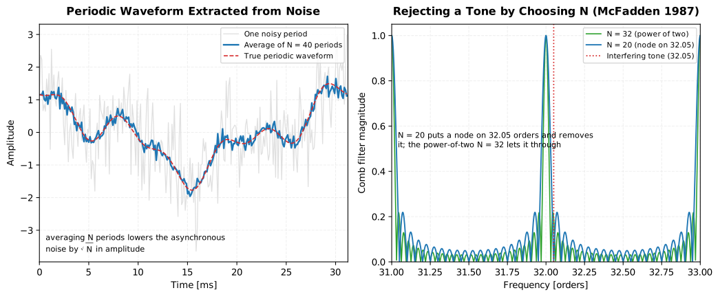
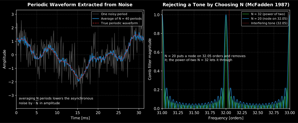
Two-panel figure. Left: one noisy period of a signal in faint grey swings far above and below a smooth curve; the average of forty periods, in blue, lies almost exactly on the dashed red true waveform, so the asynchronous noise has been removed. Right: the comb-filter magnitude across the orders between 31 and 33, with unit-height teeth at the integer orders; for N = 20 a deep node falls exactly on the interfering tone marked at 32.05 orders, whereas the power-of-two N = 32 leaves a side lobe there and lets the tone through.

Two things worth reading separately. Left, the $N$ law doing its work: the noise on one period has an rms of 0.83, and after 40 averages the averaged waveform departs from the true one by 0.138 rms — a factor 6.0 against the $40 = 6.32$ the law predicts. Right, the choice that costs nothing: at order 32.05 the comb of $N = 20$ is 6×10⁻¹⁴, while the habitual power of two $N = 32$ still passes 0.19 of the interfering tone. Twenty averages beat thirty-two here, and only because of where the node lands.

Show the code for this figure

import matplotlib.pyplot as plt
import numpy as np
from phonometry import (
    comb_filter_response,
    noise_signal,
    time_synchronous_average,
)

fs = 8192.0
period = 1.0 / 32.0        # one revolution: 256 samples at this rate
m, n_avg = 256, 40
phase = np.arange((n_avg + 1) * m) / m
periodic = (
    np.cos(2.0 * np.pi * phase)
    + 0.5 * np.cos(2.0 * np.pi * 3.0 * phase + 0.4)
    - 0.3 * np.cos(2.0 * np.pi * 6.0 * phase)
)
recording = periodic + noise_signal(fs, phase.size / fs, rms=0.9, seed=11)
res = time_synchronous_average(recording, fs, period, n_averages=n_avg)

fig, (ax0, ax1) = plt.subplots(1, 2, figsize=(11, 4.6))
t_ms = 1e3 * res.times
ax0.plot(t_ms, recording[:m], color="#cccccc", label="One noisy period")
ax0.plot(t_ms, res.period_waveform, color="#1f77b4", lw=1.8,
         label=f"Average of N = {n_avg} periods")
ax0.plot(t_ms, periodic[:m], "--", color="#d62728", label="True waveform")
ax0.set_xlabel("Time [ms]"); ax0.set_ylabel("Amplitude"); ax0.legend()

orders = np.linspace(31.0, 33.0, 4000)
freqs = orders / period
ax1.plot(orders, comb_filter_response(freqs, period, 32), color="#2ca02c",
         label="N = 32 (power of two)")
ax1.plot(orders, comb_filter_response(freqs, period, 20), color="#1f77b4",
         label="N = 20 (node on 32.05)")
ax1.axvline(32.05, color="#d62728", ls=":", label="Interfering tone")
ax1.set_xlabel("Frequency [orders]"); ax1.set_ylabel("Comb filter magnitude")
ax1.set_ylim(0, 1.05); ax1.legend()
plt.show()

The .plot() method draws the averaged waveform and the comb filter in one call:

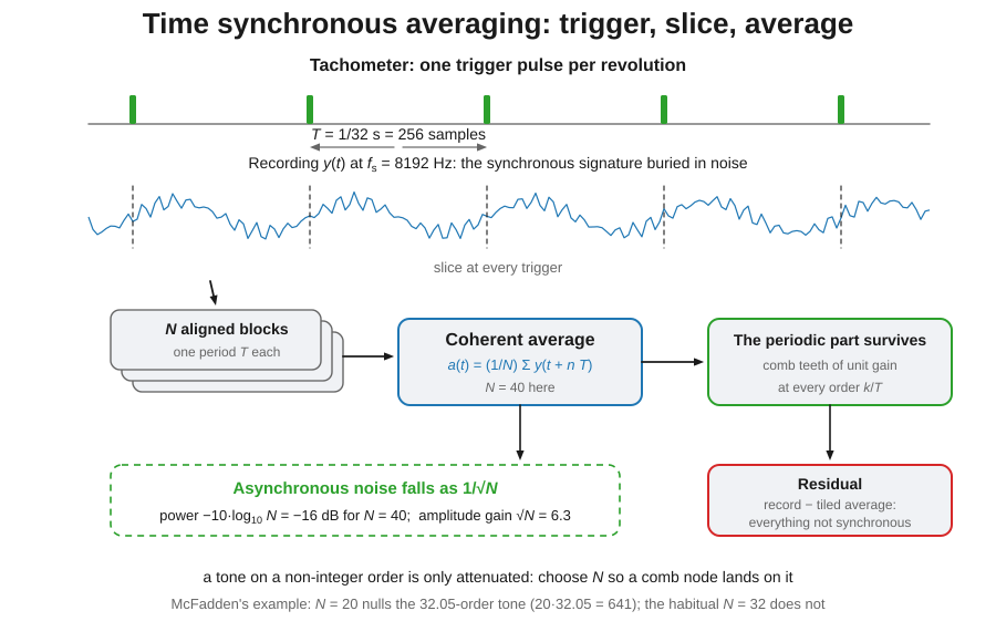
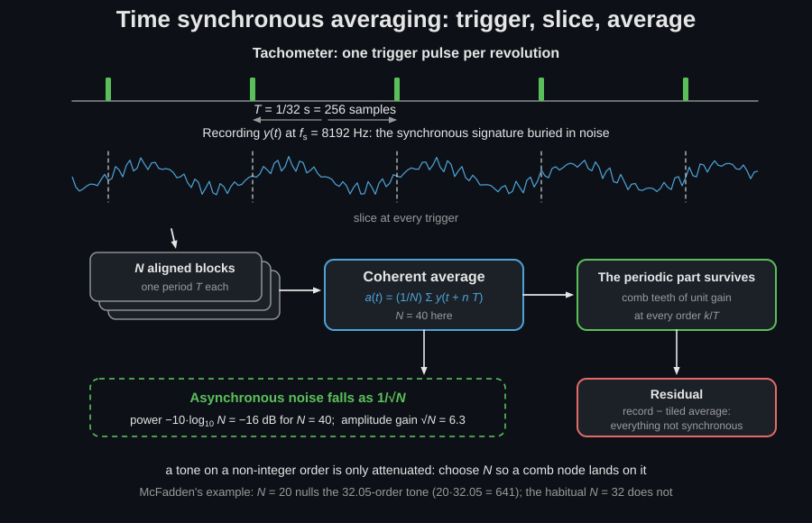
res.plot()          # English labels; res.plot(language="es") for Spanish

Before the algebra, the procedure itself: a trigger marks each revolution, the record is sliced at every trigger, and the aligned blocks are averaged: what repeats with the period survives intact while asynchronous content is attenuated.

Block diagram of time synchronous averaging: a tachometer delivers one trigger pulse per revolution with period T equal to 1 over 32 seconds, 256 samples at 8192 hertz, the noisy recording is sliced at every trigger into N aligned one-period blocks, and their coherent average, N equal to 40 here, keeps the periodic part with unit comb-filter gain at every order k over T; a dashed note quantifies that asynchronous noise power falls by 10 log N equal to 16 decibels for N equal to 40, an amplitude gain of 6.3, while a residual box holds the record minus the tiled average; the caption recalls McFadden's rule that N equal to 20 places a comb node exactly on a 32.05 order interfering tone while the habitual N equal to 32 does not

1. The average is a comb filter

Averaging $N$ successive periods (McFadden Eq. 5),

a (t) = \frac{1}{N} n = 0 \sum N - 1 y (t + n T),

is, in the frequency domain, the multiplication of the signal spectrum by a comb filter (Eq. 8). Its magnitude (Eq. 9) is the Dirichlet kernel

∣ C (f) ∣ = \frac{sin ( N π f T )}{N sin ( π f T )} .

The comb has a tooth of unit height at every harmonic $k / T$ (the orders $f T = 1, 2, 3, \dots$ ), independent of $N$ : components synchronous with the period pass untouched. Between the teeth it has nodes at $j / (N T)$ for every $j$ that is not a multiple of $N$ , where the response is exactly zero. comb_filter_response evaluates this closed form directly:

import numpy as np
from phonometry import comb_filter_response

period = 1.0 / 32.0
comb_filter_response(np.array([16.0 / period]), period, 8)   # 1.0 at a tooth
comb_filter_response(np.array([0.25 / period]), period, 2)   # 1/sqrt(2)
comb_filter_response(np.array([0.5 / period]), period, 2)    # 0.0 at a node

SynchronousAverageResult carries the response over the first few harmonics in comb_frequencies and comb_response, so the shape of the filter that the average applied is available alongside the recovered waveform.

2. Noise falls as the square root of the number of averages

Asynchronous noise of variance $σ^{2}$ averaged over $N$ periods has residual variance $σ^{2} / N$ : the residual standard deviation falls as $1/ N$ , and the amplitude signal-to-noise ratio improves by $N$ . That is a power reduction of $10 lo g_{10} N$ dB, reported as noise_reduction_db, with the amplitude gain $N$ as amplitude_snr_gain:

res = time_synchronous_average(recording, fs, period, n_averages=100)
res.noise_reduction_db      # 20.0 dB = 10*log10(100)
res.amplitude_snr_gain      # 10.0   = sqrt(100)
res.plot()                  # averaged waveform + the comb it applied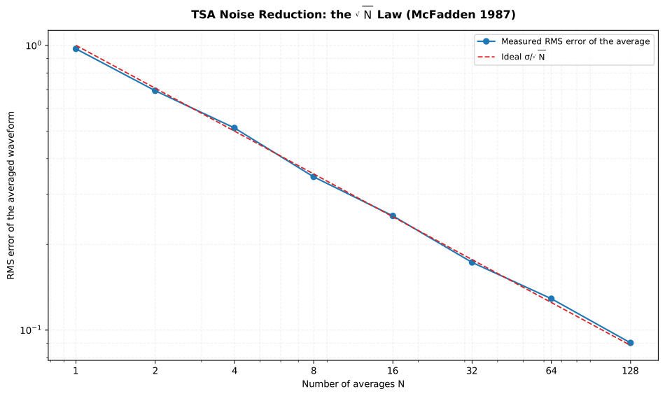

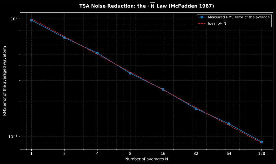
Log-log plot of the RMS error of the synchronous average against the number of averages from 1 to 128: the measured error markers fall along the dashed ideal one-over-square-root-of-N line, dropping from about 1 at a single period to below 0.1 at 128 averages

The $N$ law measured end to end: the RMS error of the averaged waveform of a three-harmonic gear signature in unit-variance noise falls along the ideal $σ / N$ line as the number of averaged periods grows from 1 to 128.

Show the code for this figure

import matplotlib.pyplot as plt
import numpy as np
from phonometry import time_synchronous_average

fs = 8192.0
samples = 256
period = samples / fs
m = np.arange(samples) / fs
true = (np.cos(2 * np.pi * m / period)
        + 0.5 * np.cos(2 * np.pi * 3 * m / period + 0.7)
        + 0.25 * np.cos(2 * np.pi * 5 * m / period + 1.1))
rng = np.random.default_rng(5)
recording = np.tile(true, 128) + rng.standard_normal(128 * samples)

counts = [1, 2, 4, 8, 16, 32, 64, 128]
errors = []
for n in counts:
    res = time_synchronous_average(recording[:n * samples], fs, period,
                                   n_averages=n)
    errors.append(np.sqrt(np.mean((res.period_waveform - true) ** 2)))

# One line — the averaged waveform and the comb filter it applied:
res.plot()
plt.show()

# The sqrt(N) law by hand: measured error against the ideal line:
fig, ax = plt.subplots()
ax.loglog(counts, errors, "o-", label="measured RMS error")
ax.loglog(counts, 1 / np.sqrt(np.array(counts)), "r--",
          label="ideal sigma/sqrt(N)")
ax.set(xlabel="Number of averages N", ylabel="RMS error")
ax.legend()
plt.show()

This law is the ideal one: it holds when the noise is uncorrelated from one period to the next, so colored or synchronous noise that is correlated across periods need not follow it. The residual (input minus the periodic reconstruction over the analysed span) and its residual_rms therefore report the noise actually left once the synchronous component is removed.

3. Choosing N to reject an interfering order

Because a tooth sits on every integer order, TSA passes the harmonics of the target shaft but also any tone that happens to fall on an integer order. A tone at a non-harmonic order $q = f T$ is only attenuated by the comb, not removed, and how much depends on where the nearest node lands. McFadden’s revised-model result is that such an interferer is best rejected by choosing $N$ so that a node falls exactly on it, i.e. the smallest $N$ with $N q$ an integer, rather than by the habitual power-of-two number of averages. An exact node exists only when the order $q$ is rational, so some finite $N$ makes $N q$ an integer; for an irrational or merely estimated order, choose the $N$ whose node falls nearest the interfering order.

His own example is a tone at 32.05 orders. With $N = 20$ the product $20 \cdot 32.05 = 641$ is an integer, so a comb node lands on the tone and rejects it by more than 100 dB. The common choice $N = 32$ gives $32 \cdot 32.05 = 1025.6$ , which sits on a side lobe: the tone is barely touched. The figure above shows both combs around order 32; the end-to-end average confirms it:

# true 8th-order component plus a strong interferer at 32.05 orders
phase = np.arange(41 * 256) / 256
recording = np.cos(2 * np.pi * 8.0 * phase) + 0.7 * np.cos(2 * np.pi * 32.05 * phase)

leak_20 = time_synchronous_average(recording, fs, period, n_averages=20)
leak_32 = time_synchronous_average(recording, fs, period, n_averages=32)
# leak_20.period_waveform matches the clean 8th-order tone; leak_32 does not

So a power-of-two number of averages, convenient as it is, is not in general the optimal choice: the interfering orders present in the machine should set $N$ .

Where the period comes from, and how steady it must be

Everything above takes $T$ as given. In a real measurement $T$ has to be measured, and the assumption hiding behind a scalar period is that the shaft holds that period for the whole record — which is the dominant failure mode of the technique and fails silently.

Getting the period. Instrument the shaft with a once-per-revolution pulse: an optical sensor against a single strip of reflective tape, an inductive probe on a keyway, or the index output of an encoder. Record that channel simultaneously with the vibration, and take $T$ as the mean interval between pulses over the analysed span. Do not take it from the nameplate speed; a nameplate is a rating, not a measurement, and a machine under load is not on its nameplate.

How steady it must be. The comb algebra of section 1 answers this exactly. A relative period error $δ$ moves the $k$ -th harmonic from the comb tooth at order $k$ to order $k (1 + δ)$ , where the same Dirichlet kernel attenuates it by

\frac{sin ( π k N δ )}{N sin ( π k δ )},

so the loss grows with the harmonic number and with the number of averages — exactly the two things one wants large. Keeping that loss under 1 dB needs roughly $k N δ < 0.25$ . Averaging 40 revolutions and expecting the 10th harmonic intact therefore demands the period be right to better than $0.25/ (10 \times 40) = 6.3 \times 1 0^{- 4}$ , that is 0.06 % speed stability; the 20th order at $N = 40$ demands 0.03 %. A machine holding speed to 1 % loses everything above the first order or two, progressively, and the resulting waveform looks smooth — which reads as a healthy gear.

The remedies, in order. Take the period from the tacho rather than from the nameplate; slice on the measured pulse intervals (one average per speed plateau if the speed steps); angularly resample the record against the tacho — order tracking — before averaging when the speed drifts continuously; and failing all three, average fewer revolutions and accept the $N$ penalty, because a short average at the right period beats a long average at the wrong one.

The acceptance check. residual_rms should fall as $1/ N$ . If it stops falling, either the speed drifted or what is left is synchronous and no number of averages will remove it.

Setting up the measurement

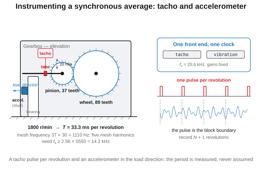
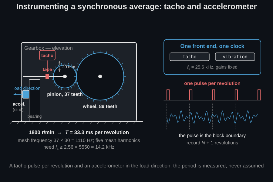
Transducer and mounting. A stud- or adhesive-mounted accelerometer on the bearing housing nearest the gear of interest, with its axis in the load direction. A magnet base collapses the usable band to a couple of kilohertz and hides the mesh harmonics the average exists to show.
Sample rate from the content you want to keep. A 37-tooth pinion at 1800 r/min meshes at $37 \times 30 = 1110$ Hz, so keeping five mesh harmonics needs $f_{s} \geq 2.56 \times 5550 = 14.2$ kHz — 16 kHz in practice, 25.6 kHz on an analyser that offers it.
Record length of $N + 1$ revolutions, with $N$ chosen by the interfering-order rule of section 3 rather than by habit.
Both channels on one simultaneously sampling front end, at a gain fixed for the whole run: a channel skew shifts every block boundary and rotates the averaged waveform.
Record the operating point — speed, load, oil temperature — because a TSA waveform is comparable only with another taken at the same one.

4. Non-integer samples per period

When $f_{s} T$ is an integer, the period boundaries fall on samples, the blocks are sliced directly, and a noiseless periodic signal is recovered to machine precision (interpolated is False). When $f_{s} T$ is not an integer the boundaries fall between samples; each block is then aligned to a common integer grid by the band-limited fractional delay of fractional_delay, and the waveform is recovered within that interpolation error (interpolated is True):

fs = 8192.0
period = 1.0 / 31.7                       # fs * period is not an integer
t = np.arange(int(40 * period * fs)) / fs
recording = np.cos(2.0 * np.pi * t / period)  # one cycle per revolution
res = time_synchronous_average(recording, fs, period)
res.interpolated                          # True: fractional-delay alignment
res.samples_per_period                    # integer samples of one period

By default the average uses as many whole periods as the record holds; pass n_averages to fix the count (for the node-selection choice of §3), and n_harmonics to set how many harmonics of $1/ T$ the returned comb response spans.

The band-limited alignment shares its kernel with the sub-sample impulse-response alignment of the test-signals page, and the recovered waveform, being exactly one period, can be tiled to reconstruct the synchronous part of the signal for subtraction or for order analysis.

Which diagnostics tool, and when

TSA, the cepstrum and the envelope spectrum answer different questions about a rotating machine, and they compose rather than compete:

TSA needs the period (a tacho pulse or a trusted shaft speed) and returns the waveform itself, one revolution of it: the tool when you want to see what a specific shaft or gear does per turn, tooth by tooth.
The cepstrum needs no reference and detects any periodic family in the spectrum (harmonics, sidebands): the tool when the period is unknown or several families overlap and must be separated.
The envelope spectrum finds periodicities of the amplitude: the tool for bearing-style faults, whose repetition rate modulates a high-frequency resonance instead of appearing as a low-frequency tone.

The composition is standard practice: average synchronously first, then subtract; the residual field is the record with the synchronous part removed, which is exactly what the envelope spectrum should be run on once the strong gear components no longer mask the modulation.

What comes out of that chain is a set of lines, and the diagnosis is carried by their frequencies rather than by their amplitudes. The kinematic families of the machine — ball-pass frequency outer and inner race, ball spin, cage, gear-mesh frequency and its shaft-rate sidebands, blade passing, motor slip and pole pass — are computed from the geometry and the shaft speed and drawn onto the measured envelope spectrum at machine fault frequencies. Because those families are expressed in orders of the shaft, the same tacho signal that fixes the averaging period fixes the family frequencies too: a speed error corrupts the averaging and the identification together.

What this guide covers

Covered
McFadden’s revised model for time domain averaging (Mechanical Systems and Signal Processing, 1987): the comb-filter description of the average (Eq. 8, magnitude Eq. 9) implemented by comb_filter_response, the square-root noise-reduction law reported as noise_reduction_db and amplitude_snr_gain, and the choice of $N$ that places a comb node on an interfering order, following the paper’s own 32.05-order example. time_synchronous_average also implements the band-limited fractional-delay alignment used when $f_{s} T$ is not an integer.
Not covered
TSA needs a known period; finding that period, or detecting periodic families without one, is the job of the cepstrum, not of this page. Locating amplitude-modulation periodicities, such as bearing faults, is the envelope spectrum, also outside this page. McFadden’s paper is not a certification standard, so there is no compliance clause to check the implementation against.

References

McFadden, P. D. (1987). A revised model for the extraction of periodic waveforms by time domain averaging. Mechanical Systems and Signal Processing, 1(1), 83-95. https://doi.org/10.1016/0888-3270(87)90085-9The comb-filter model of synchronous averaging (Eq. 8, magnitude Eq. 9), the revised finite-record model that yields an exactly periodic result, and the observation that a non-harmonic interfering order is best rejected by choosing the number of averages so that a comb node lands on it, not by the habitual power of two.

Created and maintained by José Manuel Requena Plens ORCID All projects