Measurement uncertainty (GUM and Monte Carlo)

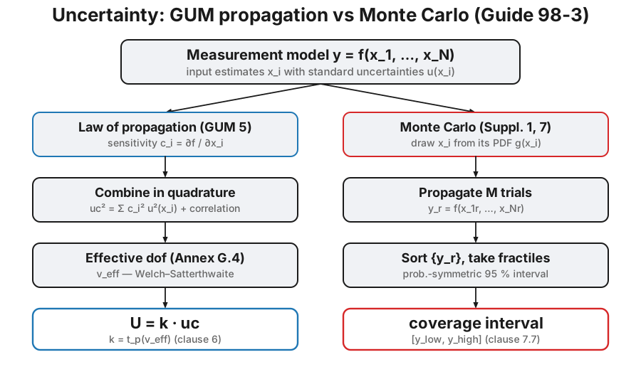
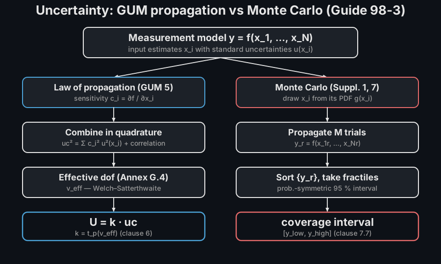
Every measurement result is incomplete without a statement of its uncertainty. The Guide to the Expression of Uncertainty in Measurement gives two ways to propagate the uncertainties of the inputs of a measurement model $y=f(x_1,\dots ,x_N)$ to the output: the law of propagation of uncertainty (JCGM 100:2008, the GUM, published also as ISO/IEC Guide 98-3:2008, clause 5) and the Monte Carlo method (JCGM 101:2008, Supplement 1, published also as ISO/IEC Guide 98-3-1:2008, clause 7). Four designations, two documents; the rest of this page says “the GUM” and “Supplement 1”. The first combines standard uncertainties analytically through the sensitivity coefficients; the second propagates the whole probability distributions numerically. They agree for linear models and diverge, informatively, when the model is non-linear or the inputs are far from Gaussian.

1. The law of propagation of uncertainty (GUM clause 5)

For a model $y=f(x_1,\dots ,x_N)$ with uncorrelated inputs, the combined standard uncertainty is the quadrature sum of the input contributions $u_i(y)=|c_i|u(x_i)$ weighted by the sensitivity coefficients $c_i=\partial f/\partial x_i$:

$$u_c^2(y)=\sum _{i=1}^N{\left(\frac{\partial f}{\partial x_i}\right)}^2{u}^2(x_i).$$

combine_uncertainty evaluates the sensitivities by central differences, so almost any callable model works, with no hand-derived partials. Input quantities are described by a Quantity (best estimate, standard uncertainty, PDF, degrees of freedom).

The step of that difference is the input’s own standard uncertainty, which is what the GUM recommends (5.1.4 NOTE 2), so the coefficient is the average slope over the range the input actually explores rather than the tangent at the estimate. For a smooth model that is a feature. It breaks on models that are not smooth over that range, and the failure is silent: a max(), a min() or a threshold — a clamp at a physical bound, a pass/fail correction — has one derivative on one side and another on the other; a table lookup or a rounded intermediate can return a sensitivity of exactly zero; a model that draws its own random numbers returns pure noise. Two defences: compare result.sensitivities against the analytic partials wherever you know them, and reach for monte_carlo whenever the model is non-smooth, because propagating distributions needs no derivative at all. The third panel of the figure in section 2 is exactly such a model.

Type A: uncertainty from repeated observations

The GUM’s first half is the one this page’s API makes easiest to skip. Given $n$ independent readings of the same quantity with experimental standard deviation $s$, the best estimate is their mean and the standard uncertainty of that mean is

$$u=\frac{s}{\sqrt{n}},\nu =n-1$$

(GUM 4.2.3) — exactly the pair a Quantity takes as uncertainty and dof. The Position input of the budget below is that: ten measurements at different microphone positions scattering with $s=1.1$ dB give $u=1.1/\sqrt{10}=0.35$ dB with dof=9.

Two consequences worth internalising. First, $s$ and $u$ describe different things: $s$ is a property of the sound field and does not shrink when you measure more positions, while $u$ does — so more positions is the only lever on this term, and it is a $\sqrt{n}$ lever. Second, a small $n$ is expensive twice: once through $\sqrt{n}$, and once through the coverage factor, because 9 degrees of freedom already lift $k$ from 1.96 to 2.11 and 4 degrees of freedom lift it to 2.78. Entering the raw $s$ instead of $s/\sqrt{n}$, or leaving dof at its infinite default, are the two commonest ways to get this term wrong, and they pull in opposite directions.

Type B: uncertainty from a stated bound

Type B evaluations start from a half-width $a$ — a tolerance, a resolution, a manufacturer’s limit — and a choice of distribution over it (GUM clause 4.3):

Constructor	$u$	Use when
rectangular(x, a)	$a/\sqrt{3}$	only bounds are known and nothing inside them: a class tolerance, a display resolution, a stated limit. The honest default
triangular(x, a)	$a/\sqrt{6}$	values near the centre are demonstrably more likely than values at the edges: the sum of two comparable rectangular influences, a quantity that was centred by adjustment
u_shaped(x, a)	$a/\sqrt{2}$	the influence cycles through its range and spends most of its time at the extremes: a thermostatted room swinging between switching points, a standing-wave field sampled at an arbitrary position

The two Type B inputs of the budget below are both bounds, hence both rectangular: the 0.20 dB calibration half-width is the calibrator’s class tolerance together with the pre/post drift observed in the field check, and the 0.30 dB instrument half-width is the meter’s class tolerance at the reference frequency. The choice of distribution reaches the GUM result only through $u$, so the same half-width read as triangular would simply divide by $\sqrt{6}$; but it sets the shape of the Monte Carlo output entirely, which is why the two methods agree on this budget and would not if one rectangular term dominated it — the first panel of the figure in section 2.

from phonometry import metrology

# A-weighted level: a reading plus zero-mean calibration, instrument and
# positional corrections. The model is their sum.
quantities = [
    metrology.Quantity(74.0, 0.0, name="Reading"),
    metrology.rectangular(0.0, 0.20, name="Calibration"),
    metrology.rectangular(0.0, 0.30, name="Instrument"),
    metrology.Quantity(0.0, 0.35, dof=9, name="Position (Type A)"),
]
result = metrology.combine_uncertainty(lambda a, b, c, d: a + b + c + d, quantities)

print(round(result.value, 2))                 # 74.0
print(round(result.combined_uncertainty, 3))  # 0.407 dB
print(result.contributions.round(3))          # [0.    0.115 0.173 0.35 ]
print(round(result.effective_dof, 1))         # 16.5

k, U = result.expanded(0.95)
print(round(k, 2), round(U, 2))               # 2.11 0.86  ->  Y = 74.0 ± 0.9 dB

Reading the budget you just computed

A budget is a decision aid, not a certificate, and this one says something specific in one glance. The position term contributes 0.350 dB of the 0.407 dB total, which is 74 % of the variance on its own; instrument and calibration together are the remaining 26 %; the reading itself contributes nothing, because it carries no uncertainty of its own in this model. The measurement is limited by where the microphone was, not by the instrument.

Quadrature makes that lesson quantitative and slightly brutal. Removing the calibration term altogether — a perfect calibrator, no drift — moves $u_c$ from 0.407 to 0.390 dB, a gain of 0.017 dB for an impossible effort. Halving the position term instead, which means four times as many positions, moves it to 0.272 dB. Budgets are improved at the top of the bar chart and never at the bottom, and the bar chart is there to tell you which end is which.

Finally, calibrate your expectations for the number itself. An expanded uncertainty near 1 dB is the ordinary outcome for a class 1 chain and a handful of positions. Standardized budgets for environmental and occupational measurements land between 1 and 3 dB once source, meteorological and sampling terms enter. Anything much below half a decibel should prompt a search for the term that was left out rather than satisfaction.

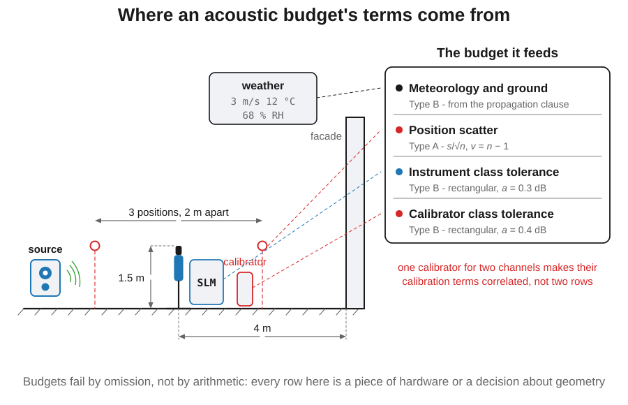
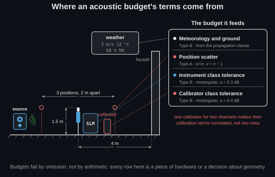
Every row of a budget is a piece of hardware or a decision about geometry, and budgets go wrong by omission far more often than by arithmetic: the forgotten meteorological term, the forgotten mounting or directivity term, the calibrator term counted twice as though the two channels had been calibrated independently.

Coverage factor and effective degrees of freedom

The expanded uncertainty $U=k{u}_c$ scales the combined uncertainty by a coverage factor $k=t_p({\nu }_{\text{eff}})$ from the $t$-distribution at the effective degrees of freedom given by the Welch–Satterthwaite formula (Annex G.4). Here the single Type A input (9 degrees of freedom) pulls ${\nu }_{\text{eff}}$ down to 16.5, so $k=2.11$ rather than the large-sample 1.96. This chain reproduces the GUM’s own worked examples end to end: the Annex H.1 end-gauge budget ($u_c=31.7$ nm, $U_{99}=92$ nm against the printed 32/93) and the Annex H.2 correlated resistance measurement ($u_c(R)=0.071\Omega$, $u_c(X)=0.295\Omega$, $u_c(Z)=0.236\Omega$ from Table H.3).

expanded(0.95) implements the GUM’s own rule: a two-sided interval with $k$ taken from the $t$-distribution at ${\nu }_{\text{eff}}$. Acoustics standards routinely fix $k$ by convention instead — $k=2$ for a two-sided 95 % statement when the degrees of freedom are large, and $k=1.65$ for the one-sided 95 % statement used when a level is compared against a limit and only exceedance matters. The same $u_c=0.407$ dB then gives three different expanded uncertainties:

Convention	$k$	$U$
GUM, two-sided, $t$ at ${\nu }_{\text{eff}}=16.5$	2.11	0.86 dB
Conventional two-sided, large sample	2	0.81 dB
One-sided, against a limit	1.65	0.67 dB

A compliance decision can turn on that choice alone, so the convention belongs next to every $U$ you quote. coverage_factor_override is how to impose a standard’s prescribed $k$ — and it is also the only route when the budget is correlated, for the reason below.

Correlated inputs

Correlated inputs are handled by passing a correlation matrix; a fully correlated sum then adds linearly instead of in quadrature. Correlation is the classic silent error in a budget: two corrections traceable to the same calibrator, or two channels sharing one instrument, do not average away the way independent terms would, and combining them in quadrature as if they were uncorrelated typically understates $u_c$. With sensitivities of opposite sign the bias points the other way, and a fully correlated pair can cancel exactly.

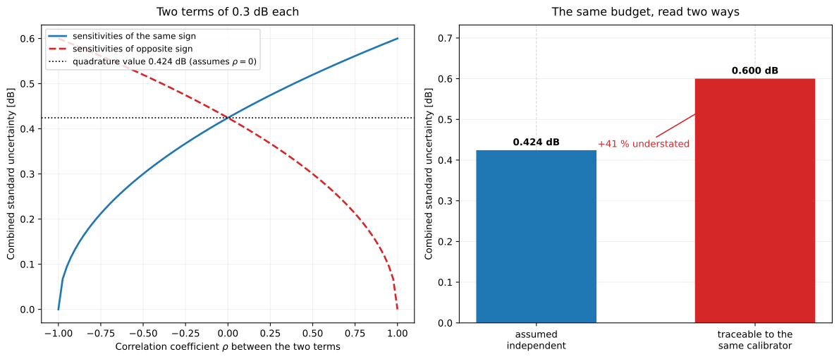
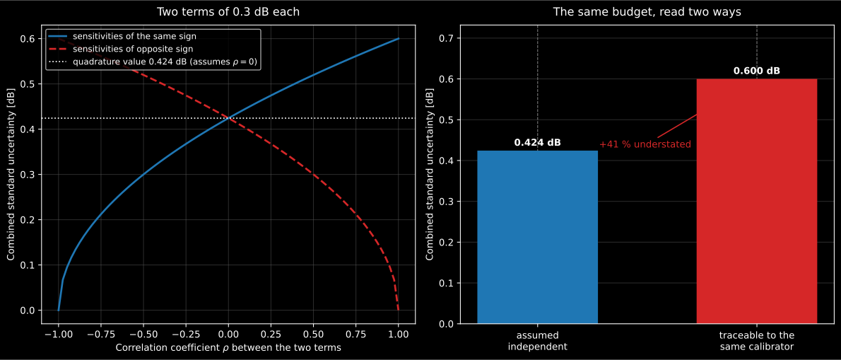
Two terms of 0.3 dB each, combined by combine_uncertainty with a correlation matrix. Treating a fully correlated pair as independent understates $u_c$ by 41 % — 0.424 dB instead of 0.600 dB — and the error grows with the number of terms that share a source. Reading the same curve backwards: a pair with $\rho =-1$ and same-sign sensitivities cancels to zero, which is what a differential measurement through one instrument buys you.

Because the GUM defines Welch–Satterthwaite for independent inputs only, a correlated budget with finite input degrees of freedom carries no effective degrees of freedom at all. What to do depends on the budget:

The budget	effective_dof	What to do
Uncorrelated	Welch–Satterthwaite value	nothing: expanded(p) takes $k$ from $t$ at ${\nu }_{\text{eff}}$
Correlated, every input Type B with infinite dof	$\infty$	nothing: $k$ comes from the normal distribution
Correlated, any input with finite dof	nan, with a warning	pass an explicit $k$: expanded(0.95, coverage_factor_override=2.0)

# Same four inputs, now with the calibration and instrument terms fully
# correlated because both are traceable to the same calibrator.
correlation = [
    [1.0, 0.0, 0.0, 0.0],
    [0.0, 1.0, 1.0, 0.0],
    [0.0, 1.0, 1.0, 0.0],
    [0.0, 0.0, 0.0, 1.0],
]
correlated = metrology.combine_uncertainty(  # warns: no Welch-Satterthwaite here
    lambda a, b, c, d: a + b + c + d, quantities, correlation=correlation)
print(round(correlated.combined_uncertainty, 3))            # 0.454 dB (was 0.407)
print(correlated.effective_dof)                             # nan
print(round(correlated.expanded(0.95, coverage_factor_override=2.0)[1], 2))  # 0.91

Counting the shared calibrator once instead of twice costs 0.047 dB here, on a budget where the two Type B terms are small. On a budget where they dominate — a two-channel intensity measurement, a level difference between two rooms measured with one meter — the same mistake is the 41 % of the figure above.

2. The Monte Carlo method (Supplement 1)

When the model is non-linear or the inputs are markedly non-Gaussian, the GUM Gaussian assumption for the output can be inaccurate. monte_carlo instead draws samples of each input from its PDF, evaluates the model over all trials and reports the mean, the standard deviation and the probabilistically symmetric coverage interval (equal probability in each tail, clause 7.7). The inputs are sampled independently; the Supplement’s multivariate-Gaussian path for non-independent quantities (6.4.8) is not implemented, so correlated budgets belong to combine_uncertainty. The number of trials is fixed (no adaptive 7.9 procedure, at least 2 trials) and the interval is the symmetric one, not the 5.3.4 shortest interval.

from phonometry import metrology

quantities = [
    metrology.Quantity(74.0, 0.0, name="Reading"),
    metrology.rectangular(0.0, 0.20, name="Calibration"),
    metrology.rectangular(0.0, 0.30, name="Instrument"),
    metrology.Quantity(0.0, 0.35, dof=9, name="Position (Type A)"),
]
mc = metrology.monte_carlo(lambda a, b, c, d: a + b + c + d, quantities,
                    trials=1_000_000, coverage=0.95, seed=1)

print(round(mc.value, 2))                 # 74.0
print(round(mc.standard_uncertainty, 3))  # 0.407 dB  (matches uc above)
print([round(x, 2) for x in mc.interval]) # [73.2, 74.8]

For this near-linear model the Monte Carlo standard uncertainty reproduces the GUM $u_c$ to three digits and the 95 % interval matches $Y\pm U$. The two methods are validated against the Guides’ own worked examples: the additive model of four unit inputs gives $u_c=2.0$ (Supplement 1 clause 9.2), and four rectangular inputs give a Monte Carlo interval of $[-3.88,3.88]$ (Supplement 1 clause 9.2.3).

When does the Monte Carlo method earn its extra cost? Whenever either of the GUM’s two simplifications fails: the model is replaced by its first-order expansion, and the output distribution by a Gaussian (or a $t$). Both hold well for the additive level model above, which is why the two methods agree to three digits. They stop holding when the model is strongly non-linear over the span of the input uncertainties (energy-to-level conversions with wide inputs, products and quotients with large relative uncertainties), when a single non-Gaussian input dominates the budget (one large rectangular term makes the output nearly rectangular, and a Gaussian $\pm 2u_c$ interval overcovers it), or when the output sits near a physical bound (an absorption coefficient near 0 or 1, a level correction that cannot cross zero), where the true coverage interval is asymmetric and no $Y\pm U$ statement can represent it. In those regimes the Monte Carlo interval is the reference: Supplement 1 (clause 8) treats the GUM framework as validated precisely when it agrees with the Monte Carlo result, and as superseded by it when it does not.

Those three regimes are worth seeing rather than being told about, because a reader who has never watched a GUM interval fail cannot recognise the failure in a budget of their own:

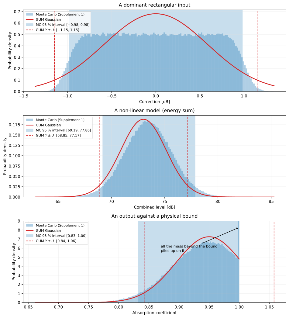
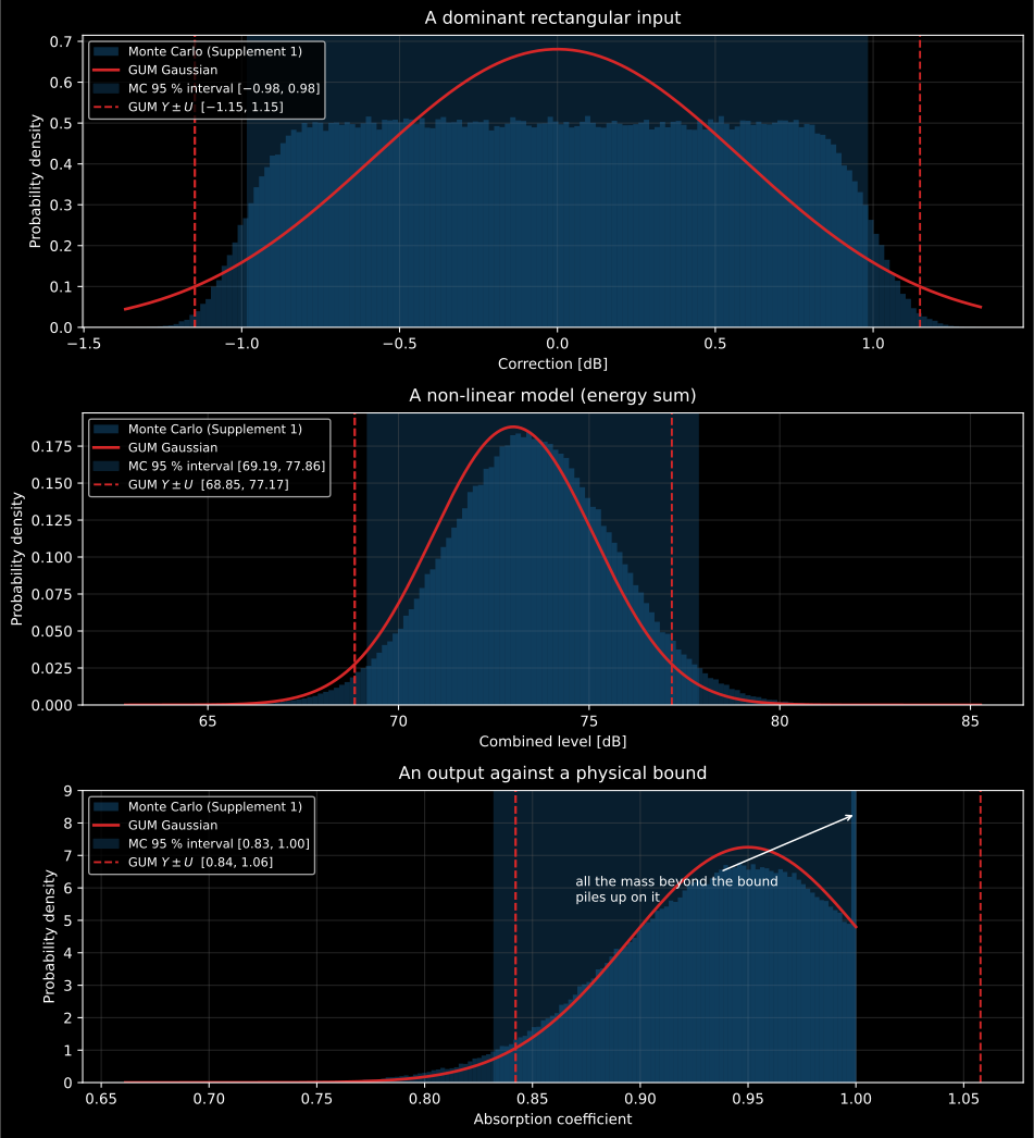
The three regimes, each computed with combine_uncertainty and monte_carlo on the same inputs. Top, one dominant rectangular term ($a=1$ dB) beside a small Gaussian one: the output is nearly rectangular, and the GUM interval $\pm 1.15$ dB overcovers the Monte Carlo $[-0.98,0.98]$ by 17 %. Middle, the energy sum $10{\log }_{10}(10^{L_1/10}+10^{L_2/10})$ of two levels with $u=3$ dB each: the Monte Carlo distribution is skewed and its mean, 73.48 dB, sits 0.47 dB above the value the GUM propagates through the model, 73.01 dB — the first-order expansion has lost a real bias. Bottom, an absorption coefficient of 0.95 with $u=0.06$ against the physical bound at 1: the GUM interval reaches 1.06, which does not exist, while the Monte Carlo interval $[0.83,1.00]$ is asymmetric and no $Y\pm U$ statement can express it. In all three, Supplement 1 clause 8 says the Monte Carlo result is the reference.

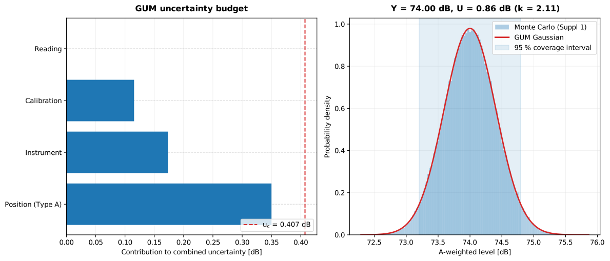
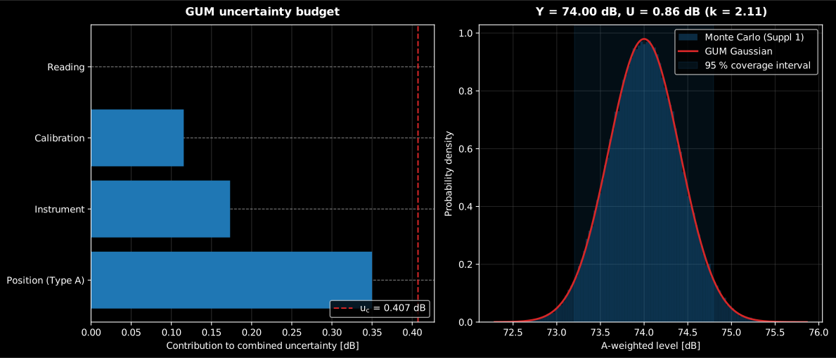
Left is where the money goes: the ten positions carry 73.9 % of the variance on their own, the instrument 18.1 % and the calibrator 8.0 %, so $u_c$ = 0.407 dB is a statement about the survey design and not about the meter. Halving the instrument term would move $u_c$ by 0.02 dB; three more positions move it by ten times that. Right is the same budget resampled a million times: the Monte Carlo standard uncertainty is 0.4073 dB against the GUM’s 0.4072, and its 95 % interval $[73.20,74.80]$ matches $Y\pm U$ = 74.00 ± 0.86 dB with $k=2.115$ at ${\nu }_{\text{eff}}$ = 16.5 — this is the near-linear case where the two methods agree, and the panel above shows the three where they do not.

Show the code for this figure

import matplotlib.pyplot as plt
import numpy as np
from phonometry import metrology

quantities = [
    metrology.Quantity(74.0, 0.0, name="Reading"),
    metrology.rectangular(0.0, 0.20, name="Calibration"),
    metrology.rectangular(0.0, 0.30, name="Instrument"),
    metrology.Quantity(0.0, 0.35, dof=9, name="Position (Type A)"),
]
model = lambda a, b, c, d: a + b + c + d
result = metrology.combine_uncertainty(model, quantities)
mc = metrology.monte_carlo(model, quantities, trials=1_000_000, coverage=0.95, seed=1,
                    keep_samples=True)
k, U = result.expanded(0.95)

# One line per panel — the budget bars, and the Monte Carlo histogram with
# its coverage interval (the committed figure also overlays the GUM Gaussian):
result.plot()
mc.plot()
plt.show()

# By hand, both panels — budget bars and the Monte Carlo output distribution:
fig, (ax1, ax2) = plt.subplots(1, 2, figsize=(12.5, 5.4))
ax1.barh(result.names, result.contributions)
ax1.axvline(result.combined_uncertainty, ls="--",
            label=rf"$u_\mathrm{{c}}$ = {result.combined_uncertainty:.3f} dB")
ax1.invert_yaxis(); ax1.legend()

rng = np.random.default_rng(1)
samples = model(np.full(200_000, 74.0),
                rng.uniform(-0.20, 0.20, 200_000),
                rng.uniform(-0.30, 0.30, 200_000),
                rng.normal(0.0, 0.35, 200_000))
ax2.hist(samples, bins=120, density=True, alpha=0.35, label="Monte Carlo")
ax2.axvspan(*mc.interval, alpha=0.12, label="95 % coverage interval")
ax2.set_title(f"Y = {result.value:.2f} dB,  U = {U:.2f} dB (k = {k:.2f})")
ax2.legend()
plt.show()

The UncertaintyResult carries the value, combined_uncertainty, the sensitivities, the per-input contributions and the effective_dof; its .plot() draws the budget and .expanded(coverage) returns the pair $(k,U)$. The MonteCarloResult carries the value, standard_uncertainty, the coverage interval and its coverage; with keep_samples=True it also retains the output samples, and its .plot() draws the output histogram with the coverage interval marked (the right panel above). The building-acoustics uncertainty of ISO 12999-1, which combines reproducibility terms for a single-number rating, is a separate, domain-specific budget.

A budget is only as honest as the record behind it: every averaged input assumes stationarity, and Data qualification provides the Bendat & Piersol tests that check it before the propagation starts.

Where the library consumes this machinery

The domain pages carry their own, standard-prescribed uncertainty clauses, and each is an instance of the clause-5 sum this page implements in general form; use this page whenever your measurement model is not one of those standardized cases:

• Calibration. The calibrator’s class tolerance and the pre/post drift bound of Calibration are textbook Type B inputs. Both are stated as half-widths, so build them with rectangular, which applies the $a/\sqrt{3}$ divisor for you: metrology.rectangular(0.0, 0.4, name="Calibrator class 1") for the IEC 60942 tolerance limit, and metrology.rectangular(0.0, d / 2, name="Drift") for a pre/post difference $d$. Do not pass a half-width to Quantity, whose second argument is already a standard uncertainty — that overstates the term by a factor 1.73 and nothing downstream will notice.
• Environmental levels. The ISO 1996-2 combined uncertainty of the Environmental Levels page is Formula (2) of that standard: the same quadrature sum with the standard’s own sensitivity coefficients.
• Building acoustics. The per-band and single-number uncertainties of field insulation measurements apply the tabulated reproducibility terms of ISO 12999-1, a standardized budget for one specific model.
• Absorption. The absorption-measurement page carries the ISO 12999-2 absorption uncertainty, the same construction for the reverberation-room method.
• Occupational exposure. The ISO 9612 uncertainty of occupational measurements budgets sampling, instrument and position contributions in exactly this way.

What this guide covers

• Covered

  From the GUM: the clause 5 law of propagation with sensitivity coefficients evaluated numerically, the clause 4.2 Type A evaluation as the uncertainty/dof pair of a Quantity, the clause 4.3 Type B evaluations (rectangular, triangular, u_shaped), correlated inputs through a correlation matrix, the Annex G.4 Welch–Satterthwaite effective degrees of freedom and the Annex G coverage factor — validated against the Annex H.1 end-gauge and Annex H.2 resistance budgets. From Supplement 1: Monte Carlo propagation of distributions with the clause 7.7 probabilistically symmetric coverage interval, checked against the clause 9.2 worked examples.

• Not covered

  The adaptive trial-count procedure of Supplement 1 clause 7.9 (the number of trials is fixed, with a minimum of 2), the shortest coverage interval of clause 5.3.4, and the multivariate-Gaussian sampling of clause 6.4.8 — so a correlated budget stays with combine_uncertainty. Supplement 2 (multiple output quantities) is not implemented at all. The clause 8 validation of the GUM framework against the Monte Carlo result is a comparison you make by reading the two results, not an automated verdict. Domain budgets prescribed by acoustics standards (ISO 1996-2, ISO 12999-1 and -2, ISO 9612) are implemented on their own pages, listed above, and are not derived here.

See also

• Data qualification: the stationarity checks every averaged input silently assumes.
• Calibration: the tolerance and drift inputs of every calibrated chain.
• API reference: metrology.uncertainty.
• Theory: Measurement uncertainty (GUM): the law of propagation of uncertainty, the coverage factor and where the Monte Carlo supplement takes over.

References

• International Organization for Standardization. (2020). Acoustics — Determination and application of measurement uncertainties in building acoustics — Part 1: Sound insulation (ISO 12999-1:2020). The domain-specific reproducibility budget for building-acoustics single-number ratings, a separate companion to the general GUM machinery.
• Joint Committee for Guides in Metrology. (2008). Evaluation of measurement data — Guide to the expression of uncertainty in measurement (JCGM 100:2008, the GUM). BIPM. https://doi.org/10.59161/JCGM100-2008EThe law of propagation of uncertainty (clause 5), Type B evaluation (clause 4.3), the expanded uncertainty and coverage factor (clause 6, Annex G), the Welch–Satterthwaite effective degrees of freedom (Annex G.4) and the Annex H worked examples that section 1 implements and reproduces. Also published as ISO/IEC Guide 98-3:2008, Uncertainty of measurement — Part 3: Guide to the expression of uncertainty in measurement (GUM:1995). The linked PDF is the free download.
• Joint Committee for Guides in Metrology. (2008). Evaluation of measurement data — Supplement 1 to the "Guide to the expression of uncertainty in measurement" — Propagation of distributions using a Monte Carlo method (JCGM 101:2008). BIPM. https://doi.org/10.59161/JCGM101-2008The Monte Carlo propagation of section 2, its probabilistically symmetric coverage interval (clause 7) and the clause 8 validation of the GUM framework against the Monte Carlo result. Also published as ISO/IEC Guide 98-3-1:2008. The linked PDF is the free download.