Multiple and partial coherence

Key references: Bendat & Piersol 2010

When several partially correlated sources drive one response, the ordinary coherence of each source with the output is misleading. A source that only correlates with the true cause inherits a spurious coherence through it, so reading the ordinary coherences alone can credit the wrong source. Bendat & Piersol, Random Data (4th ed., 2010, Chapter 7), resolve this for a multiple-input/single-output (MISO) system with the multiple and partial coherence functions. miso_coherence computes them from the same Welch cross-spectral core as the rest of phonometry.signals, for several correlated inputs and one output.

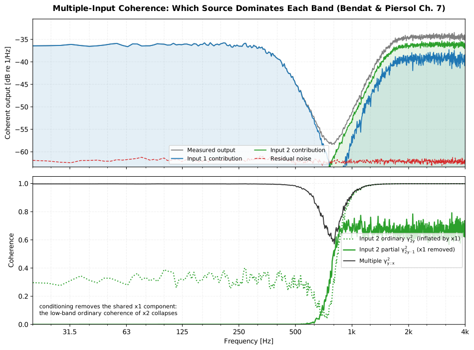
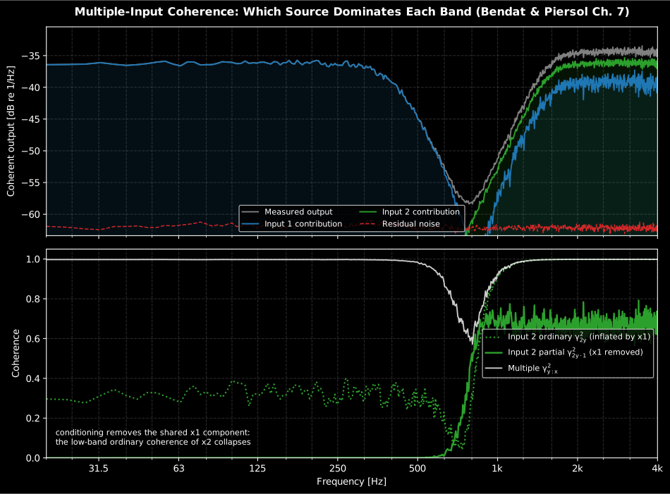
Two-panel figure. Top: the measured output autospectrum in dB with the coherent output contribution of two inputs shaded underneath; input 1 fills the low band up to about 400 Hz and input 2 fills the high band above about 1.5 kHz, with the residual noise far below. Bottom: for the correlated second input, its ordinary coherence sits around 0.3 across the low band even though it drives no low-frequency path, while its partial coherence collapses to zero there once the first input is conditioned out; the multiple coherence stays near one except at the crossover null.

The whole case for the chapter, in one measurement. Input 2 drives nothing below 400 Hz, yet its ordinary coherence with the output averages 0.324 there, inherited entirely through its correlation with input 1. Condition input 1 out and its partial coherence in the same band falls below 1×10⁻⁴ — at 200 Hz, 2.6×10⁻⁶. Multiple coherence stays at 0.997 across that band, so the model is not at fault: an engineer reading the ordinary coherences alone would spend money quietening the wrong source.

Show the code for this figure

import matplotlib.pyplot as plt
import numpy as np
from scipy import signal
from phonometry import miso_coherence, noise_signal

fs = 8192.0
# Input 1 drives a low-frequency path; input 2 = 0.7*x1 + independent noise
# drives a high-frequency path, so input 2 is correlated with input 1.
x1 = noise_signal(fs, 32.0, color="white", seed=1)
x2 = 0.7 * x1 + noise_signal(fs, 32.0, color="white", seed=2)
low = signal.butter(4, 400.0, fs=fs, output="sos")
high = signal.butter(4, 1500.0, btype="high", fs=fs, output="sos")
noise = noise_signal(fs, 32.0, color="white", rms=0.05, seed=3)
y = signal.sosfilt(low, x1) + signal.sosfilt(high, x2) + noise

res = miso_coherence([x1, x2], y, fs, nperseg=2048)
f = res.frequencies
band = (f >= 20.0) & (f <= 4000.0)

fig, (ax_top, ax_bot) = plt.subplots(2, 1, figsize=(10, 7.4), sharex=True)
db = lambda v: 10 * np.log10(v)
ax_top.semilogx(f[band], db(res.output_psd[band]), color="gray",
                label="Measured output")
for i, color in ((0, "#1f77b4"), (1, "#2ca02c")):
    ax_top.semilogx(f[band], db(res.coherent_output_spectra[i][band]),
                    color=color, label=f"Input {i + 1} contribution")
ax_top.semilogx(f[band], db(res.noise_psd[band]), "--", color="#d62728",
                label="Residual noise")
ax_top.set_ylabel("Coherent output [dB re 1/Hz]")
ax_top.legend()

ax_bot.semilogx(f[band], res.ordinary_coherence[1][band], ":", color="#2ca02c",
                label="Input 2 ordinary (inflated by x1)")
ax_bot.semilogx(f[band], res.partial_coherence[1][band], color="#2ca02c",
                label="Input 2 partial (x1 removed)")
ax_bot.semilogx(f[band], res.multiple_coherence[band], color="black",
                label="Multiple")
ax_bot.set_xlabel("Frequency [Hz]")
ax_bot.set_ylabel("Coherence")
ax_bot.set_ylim(0, 1.05)
ax_bot.legend()
plt.show()

The .plot() method draws the same two panels in one call:

res.plot()          # English labels; res.plot(language="es") for Spanish

1. Ordinary, multiple and partial coherence

For a system with $q$ inputs $x_{1} .. x_{q}$ and output $y$ , miso_coherence estimates every auto- and cross-spectrum by Welch’s method and reports three coherence functions.

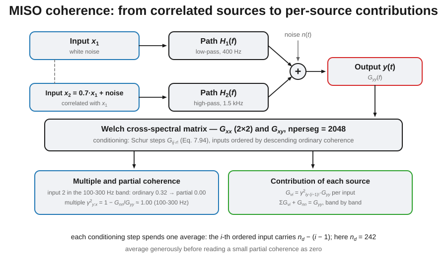
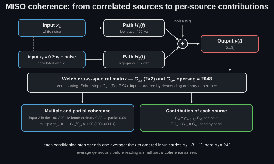
The conditioning story fits in one block diagram: two correlated inputs drive their own paths into one measured output, and the Welch cross-spectral matrix is what turns the tangle into per-source numbers.

Block diagram of a two-input MISO system: input x1 is white noise and input x2 equals 0.7 times x1 plus independent noise, x1 drives a 400 hertz low-pass path and x2 a 1.5 kilohertz high-pass path, and both sum with additive noise into the output y; the output feeds the Welch cross-spectral matrix Gxx and Gxy at nperseg 2048, conditioned by Schur steps in descending ordinary coherence order, which yields on one side the multiple and partial coherences, where input 2 in the 100 to 300 hertz band drops from an ordinary coherence of 0.32 to a partial coherence of 0.00, and on the other the per-source contributions Gvi that with the residual noise reconstruct Gyy exactly; a footnote records that each conditioning step spends one of the 242 effective averages

The ordinary coherence of input $i$ with the output, on its own (Eq. 7.109), is the familiar single-input quantity:

γ_{i y}^{2} (f) = \frac{∣ G _{i y} ( f ) ∣ ^{2}}{G _{ii} ( f ) G _{y y} ( f )} .

The multiple coherence (Eq. 7.35) is the fraction of the output autospectrum linearly explained by all inputs jointly. From the Hermitian input cross-spectral matrix $G_{xx}$ and the input-output vector $G_{x y}$ it is

γ_{y : x}^{2} (f) = \frac{G _{x y}^{H} G _{xx}^{- 1} G _{x y}}{G _{y y}} = 1 - \frac{G _{nn}}{G _{y y}},

where $G_{nn}$ is the residual output spectrum uncorrelated with every input. If the output carries additive uncorrelated noise of per-band signal-to-noise ratio $SNR$ , this is exactly $SNR / (1 + SNR)$ , the closed-form oracle used to verify the implementation.

The partial coherence of input $i$ (Eq. 7.87) is its coherence with the output once the linear effect of the inputs before it in the conditioning order has been removed. The subscript notation is the book’s, and the exclamation mark is not a factorial: a trailing $\cdot r!$ means conditioned on inputs 1 through $r$ , in the chosen order. So $G_{ij \cdot r!}$ is the cross-spectrum of $i$ and $j$ with the linear effect of the first $r$ inputs removed, and $G_{y y \cdot q!}$ — which section 2 ends on — is the output spectrum with every input removed, that is the residual noise $G_{nn}$ of the multiple coherence above. In symbols:

γ_{i y \cdot (i - 1)!}^{2} (f) = \frac{∣ G _{i y \cdot (i - 1)!} ( f ) ∣ ^{2}}{G _{ii \cdot (i - 1)!} ( f ) G _{y y} ( f )} .

The 4th-edition definition keeps the total output $G_{y y}$ in the denominator (not the conditioned output). That choice makes the partial coherences of the ordered inputs sum to the multiple coherence, $γ_{y : x}^{2} = \sum_{i} γ_{i y \cdot (i - 1)!}^{2}$ (Eq. 7.116), and reduce exactly to the ordinary coherences when the inputs are mutually uncorrelated (Eq. 7.117).

res = miso_coherence([x1, x2], y, fs)
res.ordinary_coherence   # shape (q, F): each input on its own
res.multiple_coherence   # shape (F,):  all inputs jointly
res.partial_coherence    # shape (q, F): conditioned on the preceding inputs

2. Conditioning: separating cause from correlation

The partial coherences come from the conditioned spectra $G_{ij \cdot r!}$ , computed by the Gaussian-elimination recursion of Section 7.3. Removing the linear effect of a pivot input $r$ from every remaining record is one Schur complement step (Eq. 7.94):

G_{ij \cdot r!} = G_{ij \cdot (r - 1)!} - \frac{G _{r j \cdot (r - 1)!} G _{i r \cdot (r - 1)!}}{G _{r r \cdot (r - 1)!}},

applied for each input in the conditioning order until only the residual output spectrum $G_{y y \cdot q!}$ remains. This is the whole point of the method: in the figure above, input 2 is $0.7 x_{1} + independent noise$ , so it correlates with input 1 but drives no low-frequency path. Its ordinary coherence with the output therefore reads about 0.3 across the low band, borrowed entirely through input 1, while its partial coherence collapses to zero there once input 1 is conditioned out.

low = (res.frequencies > 100.0) & (res.frequencies < 300.0)
res.ordinary_coherence[1][low].mean()   # ~0.32  (inflated through x1)
res.partial_coherence[1][low].mean()    # ~0.00  (x1 removed)

3. Which source dominates each band

The conditioning also splits the output power source by source. The partial coherent output spectrum of input $i$ (Eq. 7.86) is the share of the output autospectrum it contributes, and the shares plus the residual noise reconstruct the output exactly (Eqs. 7.88/7.121):

G_{v_{i}} = γ_{i y \cdot (i - 1)!}^{2} G_{y y}, i \sum G_{v_{i}} + G_{nn} = G_{y y} .

Comparing the shares band by band answers “which source dominates here?”. dominant_input() returns, for every frequency, the index of the input with the largest share:

res.coherent_output_spectra        # shape (q, F): Gvi per input
dominant = res.dominant_input()    # index of the strongest source per bin
f = res.frequencies
dominant[np.argmin(abs(f - 200.0))]    # 0 (input 1 drives the low band)
dominant[np.argmin(abs(f - 2500.0))]   # 1 (input 2 drives the high band)

Instrumenting a MISO measurement

Everything above runs on synthetic arrays, and the method’s whole value is on real machinery, in a real room, where the sources cannot be switched off one at a time — which is exactly why the technique exists. What it separates is what the references separate, so the reference sensors are the measurement.

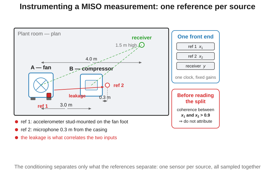
Plan view of a plant room to scale: a fan on resilient mounts and a compressor three metres apart, each with its own reference sensor, an accelerometer stud-mounted on the fan foot and a microphone 0.3 m from the compressor casing, a receiver microphone at the operator position four metres away at 1.5 m height, a dashed leakage path showing the fan's airborne sound reaching the compressor's reference microphone, and a right-hand column with the four channels entering one simultaneously sampling front end

One reference per source, placed so that it hears its own source and as little as possible of the others. An accelerometer stud-mounted on the foot of a machine, a microphone 0.2 to 0.5 m from the casing surface rather than out in the room. A reference that picks up its neighbour is the input-to-input correlation the conditioning then has to undo, and it undoes it only as far as the arithmetic allows (see below).
One simultaneously sampling front end for every reference and the receiver. The conditioning is built entirely from cross-spectra, so an inter-channel skew tilts every one of them; a converter that sequences its channels puts that skew in for free.
Fixed gains for the whole run, and every source running together at the operating point being diagnosed.
Averages to spare. Each conditioning step spends one, so the last-ordered input carries $n_{d} - (q - 1)$ ; aim for a few hundred effective averages before reading a small partial coherence as a physical zero.
Record with the result: sensor model, position and sensitivity per channel, the machine speed and load, the segment length, and the conditioning order actually applied (res.order) — the split is not reproducible without the last one.

4. Statistical quality and the conditioning order

The random errors follow Section 9.3. Conditioning on the $i - 1$ preceding inputs costs $i - 1$ degrees of freedom, so the $i$ -th ordered input carries $n_{d} - (i - 1)$ effective averages (Eqs. 9.100/9.101) and the $q$ -input multiple coherence carries $n_{d} - (q - 1)$ (Eq. 9.98). The result exposes multiple_coherence_random_error and coherent_output_random_error alongside the effective average count n_averages.

The ordinary and multiple coherences do not depend on the conditioning order, but the partial coherences and the coherent-output decomposition do: each input is conditioned on whatever precedes it. Absent a physical ordering, Bendat & Piersol (Section 7.2.4) recommend ordering the inputs by descending ordinary coherence with the output. Suppose a third, weakly coupled source is recorded alongside the two above — a fan in the next room, coherent with neither. Pass order to override the default:

x3 = noise_signal(fs, 32.0, color="white", seed=4)   # the third, weak source
res = miso_coherence([x1, x2, x3], y, fs, order=(2, 0, 1))
res.order            # (2, 0, 1): the order actually applied
res.plot()           # the two panels, recomputed in the applied order

The ordinary and multiple coherences come back identical whatever order says; the partial coherences and the per-source shares do not, because each input is credited only with what the inputs before it left unexplained.

Check the inputs against each other first

The conditioning inverts the input cross-spectral matrix, so it separates only sources that are genuinely separable. Each Schur step divides by the power the pivot input still has after the preceding inputs have been removed, so two references that are nearly the same signal leave almost nothing in that pivot and the next step amplifies estimation noise without bound. Bendat & Piersol treat the limit as its own case (their Figure 7.3): an input-to-input coherence of one means the two records are one source reaching the output by two paths, and no two-input split exists at all.

This implementation does not raise on that case. A conditioned pivot whose power falls below a relative floor is skipped, and the input contributes exactly zero — which looks identical to the page’s headline result, a source that merely correlates, even when both sources are real and only the references were badly placed.

So run the check before believing the split:

Compute the ordinary coherence between every pair of inputs — one cross_spectral_density per pair — before calling miso_coherence.
In any band where a pair exceeds about 0.9, do not read the partial coherences or the per-source shares. The multiple coherence and $G_{y y}$ are still valid there; the attribution is not.
Confirm by reordering. A well-conditioned decomposition barely moves when the inputs are reordered; an ill-conditioned one moves a lot.

The remedies are physical, not numerical: move a reference closer to its own source so it stops hearing the other one, run the sources one at a time if the machine allows it, or accept that the pair is one input and merge them.

Two further pitfalls are worth naming. Averaging: every conditioning step spends a degree of freedom, so with few segments the partial coherences of the last-ordered inputs are the least trustworthy numbers on the page; average generously before reading a small partial coherence as zero. Delay bias: like the ordinary coherence, the Welch estimate is biased low when a bulk delay between an input and the output becomes a noticeable fraction of the segment length; remove known propagation delays first (see Correlation and delay) and keep nperseg well above the longest remaining delay.

The estimators share the Welch core of the calibrated spectral analysis page (same Hann taper, 50 % overlap and detrend-off calibration), so a MISO coherence and a power_spectral_density computed with the same segment length are consistent bin by bin.

What this guide covers

Covered
Bendat & Piersol Chapter 7’s ordinary, multiple and partial coherence functions (Eqs. 7.109, 7.35, 7.87), the Gaussian-elimination conditioning recursion (Eq. 7.94), the partial coherent output spectra and their exact decomposition of the output (Eqs. 7.86/7.116/7.121), and the Section 9.3 random errors of the multiple and conditioned estimates (Eqs. 9.98-9.101), all exposed by miso_coherence and MISOCoherenceResult.
Not covered
The chapter’s multiple-input frequency-response (gain factor $L_{i y}$ ) estimates, the linear model that predicts the output from the conditioned inputs, are computed internally to build the coherent output spectra but are not returned: MISOCoherenceResult exposes the coherence and spectral-decomposition side only, not a fitted multi-input transfer function. The method is also single-output (MISO); a system with several correlated outputs needs one miso_coherence call per output.

References

Bendat, J. S., & Piersol, A. G. (2010). Random data: Analysis and measurement procedures (4th ed.). Wiley. https://doi.org/10.1002/9781118032428Chapter 7 (multiple-input/output relationships: ordinary coherence Eq. 7.109, multiple coherence Eq. 7.35, partial coherence Eq. 7.87, the conditioned-spectrum Gaussian-elimination recursion Eq. 7.94, the coherent output decomposition Eqs. 7.86/7.116/7.121) and Section 9.3 (statistical errors of the multiple and conditioned estimates, Eqs. 9.98-9.101). ISBN 978-0-470-24877-5.

Created and maintained by José Manuel Requena Plens ORCID All projects