Test signals and sample-rate tools

A measurement is only as trustworthy as its stimulus and its sample-rate bookkeeping. This page covers the signal toolbox of phonometry.signals, in the order the sections take it: tone bursts with the exact gating IEC 60268-1 prescribes, resampling whose anti-alias rejection is a stated, verifiable specification rather than a library default, fractional delay that shifts a record by any sub-sample amount with band-limited exactness, and the colored-noise generators, whose spectral verification lives in the spectral analysis guide.

Before the details, the family portrait: what each stimulus looks like in time and where its energy sits over frequency.

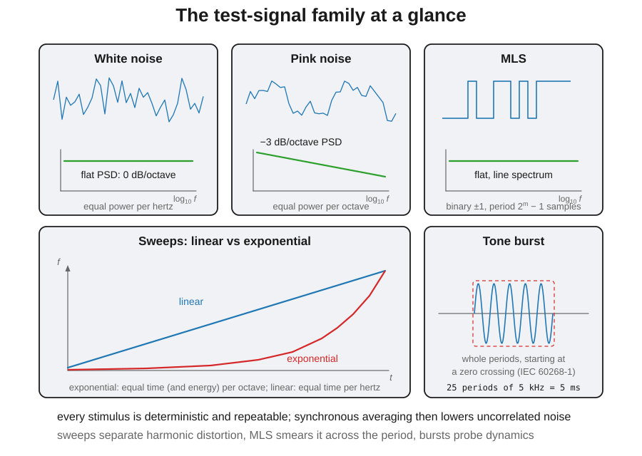
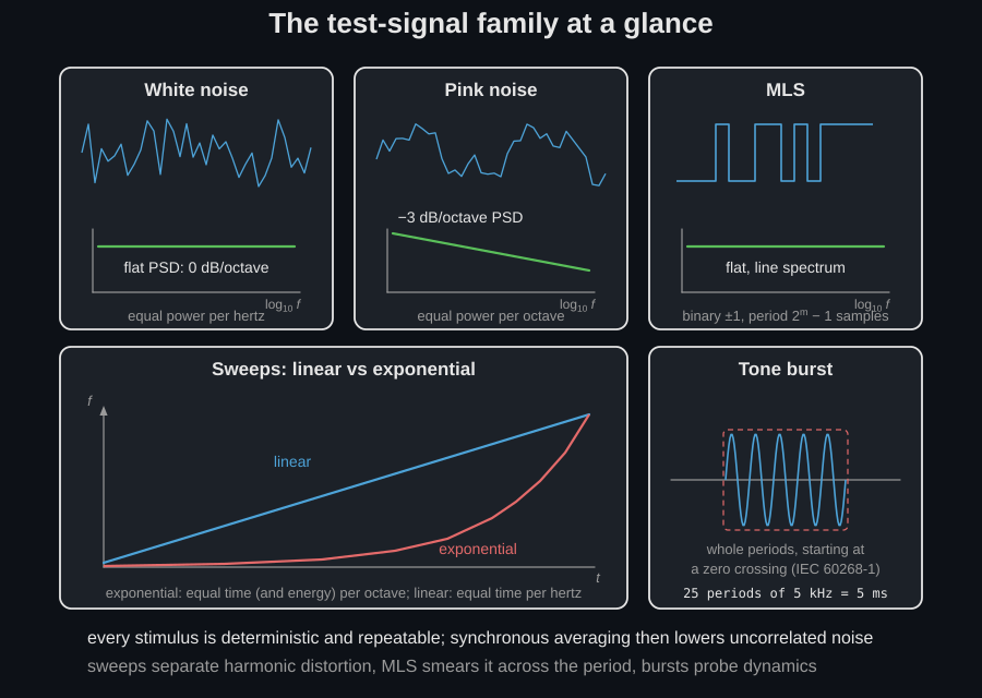
Five stimuli, and what separates them. Noise excites everything at once and needs averaging to beat its own randomness. An MLS is deterministic and periodic, so one circular cross-correlation gives an impulse response in a single pass. A sweep concentrates its energy at one frequency at a time, which is what buys both its crest factor and the separation of harmonic distortion into negative times. A gated burst probes dynamic behaviour rather than steady response.

Only two of the five are covered here, so this is where the other three live: the noise generators and their spectral verification on spectral analysis; the MLS and the exponential sweep as the ISO 18233 acquisition pair of room acoustics; the shaped sweep and the Golay pair on system measurement; and the tone burst in the next section.

1. Tone bursts (IEC 60268-1)

The gated sine burst is the standard stimulus for dynamic behaviour: sound-level-meter ballistics, quasi-peak meters, loudspeaker power handling. IEC 60268-1:1985 (Clause A2.1) pins down what a well-formed burst is: it “should start at the zero-crossing of the tone and should consist of an integral number of full periods”. tone_burst generates exactly that, as a single burst or as the repetitive train of Clause A2.2 in which each burst occupies one full repetition period:

from phonometry import tone_burst

# One 5 ms burst of 5 kHz tone (25 full periods), as in Table AII.
single = tone_burst(48000, 5000, 25)
print(single.burst_samples)         # 240 samples = 5 ms at 48 kHz

# Clause A2.2: 5 ms bursts at 10 bursts per second.
train = tone_burst(48000, 5000, 25, repetitions=4, repetition_rate=10)
print(train.period_samples, train.duty_cycle)   # 4800, 0.05
train.plot()                        # waveform with the gating envelope

The result carries the record, the rectangular gating envelope and the exact sample bookkeeping (burst_samples, onset_sample, period_samples, duty_cycle), so a test report can state its stimulus numerically. Because the gate spans an integral number of full periods starting at a zero crossing, the burst energy has the closed form $A^{2}N/2$ exactly, which is how the generator is verified.

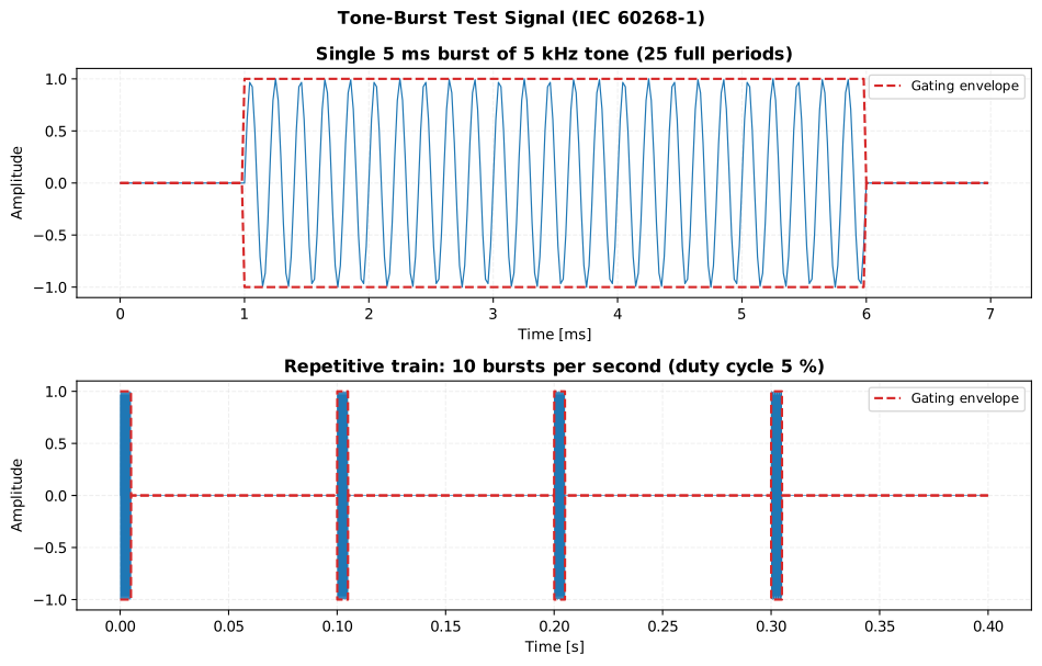
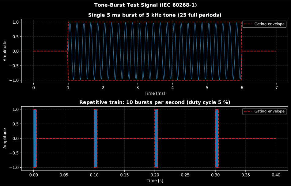
Every number in the picture is exact rather than nominal, which is the point of Clause A2.1. The burst is 240 samples, 25 full periods of 5 kHz at 48 kHz, and the first sample of the gate falls on a zero of the tone, so its energy is $A^{2}N/2=120$ to the last digit. In the train below, the period is 4800 samples and the duty cycle 0.05 exactly — the burst occupies one twentieth of each repetition, which is what makes the train usable for meter ballistics where the off time has to be as well defined as the on time.

Show the code for this figure

import matplotlib.pyplot as plt
import numpy as np
from phonometry import tone_burst

fs = 48000.0
single = tone_burst(fs, 5000, 25, pre_silence=0.001, post_silence=0.001)
train = tone_burst(fs, 5000, 25, repetitions=4, repetition_rate=10)

fig, axes = plt.subplots(2, 1, figsize=(10, 6.4))
t_ms = 1e3 * np.arange(single.signal.size) / single.fs
axes[0].plot(t_ms, single.signal, lw=0.9)
axes[0].plot(t_ms, single.envelope, "r--", label="Gating envelope")
axes[0].plot(t_ms, -single.envelope, "r--")
axes[0].set_xlabel("Time [ms]")

t_s = np.arange(train.signal.size) / train.fs
axes[1].plot(t_s, train.signal, lw=0.5)
axes[1].plot(t_s, train.envelope, "r--", label="Gating envelope")
axes[1].plot(t_s, -train.envelope, "r--")
axes[1].set_xlabel("Time [s]")

for ax in axes:
    ax.set_ylabel("Amplitude")
    ax.legend(loc="upper right")
plt.tight_layout()
plt.show()

These are the bursts behind the Fast/Slow/Impulse ballistics reference responses (IEC 61672-1 Table 4 uses 4 kHz tonebursts of 200, 50 and 10 ms) and the quasi-peak dynamic tests of IEC 60268-1 itself (5 kHz bursts of 1 to 200 ms, Table AII).

What gating does in frequency, and what the duty cycle costs in level. Multiplying a tone by a rectangle convolves its line with the gate’s transform, a sinc whose first nulls sit $1/T_{\text{burst}}$ either side of the carrier — ±200 Hz for a 5 ms burst, ±100 Hz for a 10 ms one. So it is the burst duration, not the carrier, that decides whether the stimulus fits inside a band filter, and why a short burst through a fractional-octave filter shows the filter’s own settling rather than the burst. In level, a train’s equivalent continuous level is the burst level plus $10{\log }_{10}(\text{duty cycle})$: the 5 % train above therefore sits exactly 13.0 dB below the burst’s own level, which is the quantity a detector-ballistics test compares against. The reference responses those numbers feed are in Time weighting.

2. Resampling with a stated anti-alias specification

Sample-rate conversion hides a filter, and that filter decides how much aliased energy contaminates the result. resample_signal performs rational polyphase resampling (44.1 to 48 kHz is the ratio 160/147) with a lowpass FIR designed inside the function by the Kaiser window method, from two numbers the caller controls:

• stopband_attenuation_db (default 120): the alias rejection, with the stopband starting exactly at the smaller of the two Nyquist frequencies, where folding happens;
• transition_width (default 0.05): the fraction of that Nyquist frequency given up to the filter’s transition band, so the passband ends at (1 - transition_width)·f_Nyq and is flat within the same Kaiser ripple bound $\delta =10^{-A/20}$.

from phonometry import noise_signal, resample_signal

x = noise_signal(44100, 5.0, color="pink", seed=1)
res = resample_signal(x, 44100, 48000)   # 120 dB alias rejection
print(res.up, res.down)                  # 160, 147
print(res.n_taps, res.passband_edge_hz)  # designed FIR, 20947.5 Hz
res.plot()   # the delivered anti-alias filter against its design spec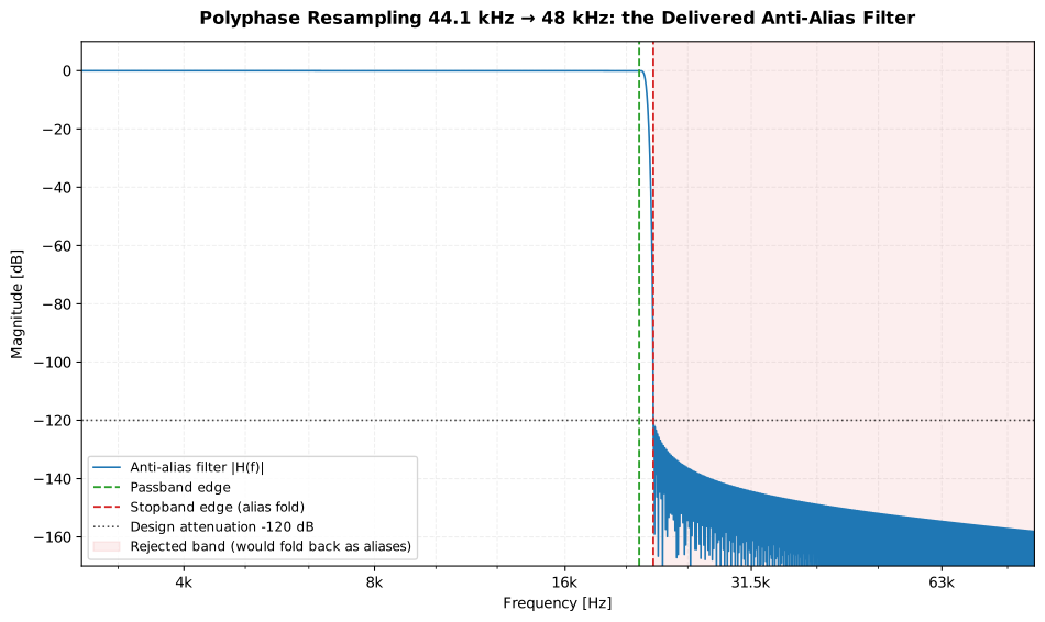

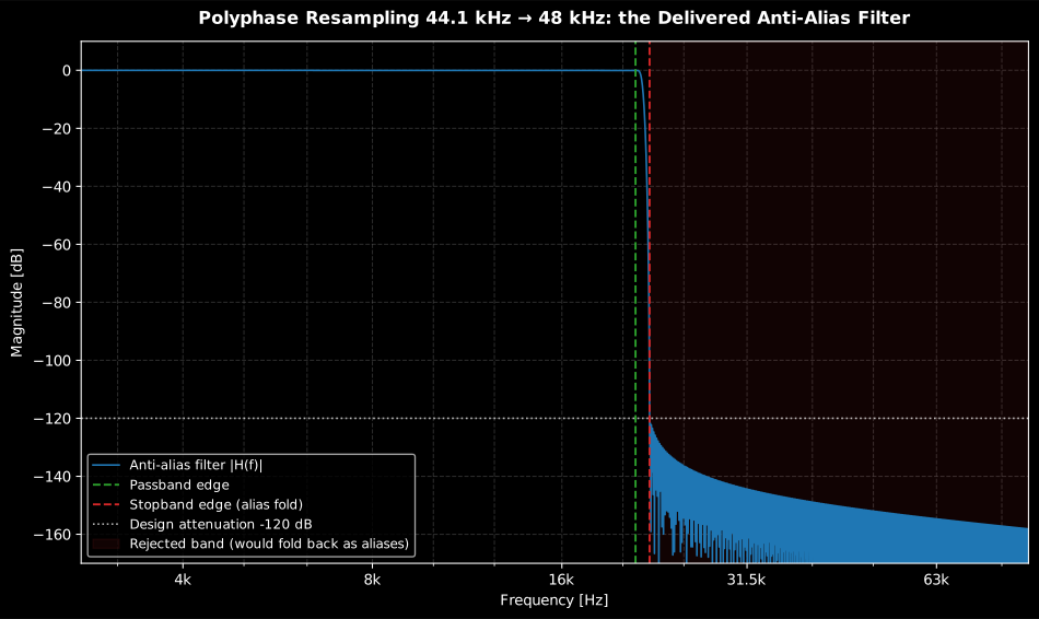
The delivered anti-alias filter of the default 44.1 → 48 kHz conversion: the stopband starts exactly at the smaller Nyquist frequency (where aliases fold) and stays below the −120 dB design line; the passband ends 5 % below it, flat within the same ripple bound.

Show the code for this figure

import matplotlib.pyplot as plt
import numpy as np
from scipy import signal
from phonometry import noise_signal, resample_signal

x = noise_signal(44100, 5.0, color="pink", seed=1)
res = resample_signal(x, 44100, 48000)   # 120 dB alias rejection

# res is the ResampledSignalResult computed in the example above.
# One line — the delivered anti-alias filter against its design spec:
res.plot()
plt.show()

# By hand, from the taps the result carries — mirroring what
# ResampledSignalResult.plot() draws:
fs_up = res.original_fs * res.up
freqs, h = signal.freqz(res.filter_taps, worN=1 << 18, fs=fs_up)
mag_db = 20 * np.log10(np.maximum(np.abs(h), 1e-300))
view = (freqs > 0) & (freqs <= 4 * res.stopband_edge_hz)

fig, ax = plt.subplots()
ax.semilogx(freqs[view], mag_db[view], label="Anti-alias filter |H(f)|")
ax.axvline(res.passband_edge_hz, color="g", linestyle="--",
           label="Passband edge")
ax.axvline(res.stopband_edge_hz, color="r", linestyle="--",
           label="Stopband edge (alias fold)")
ax.axhline(-res.stopband_attenuation_db, color="k", linestyle=":",
           label="Design attenuation -120 dB")
ax.axvspan(res.stopband_edge_hz, 4 * res.stopband_edge_hz,
           color="r", alpha=0.08)
ax.set(xlabel="Frequency [Hz]", ylabel="Magnitude [dB]")
ax.legend()
plt.show()

The designed taps travel with the result (filter_taps), so the specification is checkable: the test suite measures the frequency response of the returned filter and asserts the passband deviation and stopband leakage against the design’s own ripple bound (the design internally targets 1 dB past the request, so the delivered filter meets the stated numbers rather than a Kaiser-formula approximation of them). A passband tone resampled through the default specification matches the analytic tone at the new rate within $10^{-120/20}=10^{-6}$.

Several estimators resample internally at fixed rates (the ECMA-418-2 psychoacoustics at 48 kHz, STOI at 10 kHz); this function is the public, documented counterpart for preparing records outside those chains.

Three things worth deciding before resampling at all. The specification has a price: the default 5 % transition width gives up the top 5 % of the smaller Nyquist band, so a 44.1 → 48 kHz conversion is flat only to about 21 kHz; a record whose content reaches Nyquist needs a narrower transition_width (and the extra taps that come with it) rather than a silent truncation. Order matters: resampling is a filtering operation, so RMS-based levels survive it while peak-based ones do not — band-limited interpolation can place a reconstructed sample above the original peak (the intersample-peak effect), so lc_peak and any crest factor belong at the original rate, or behind an explicit true-peak oversampling. And often the answer is not to resample: the library’s fractional-octave filters design themselves at whatever rate they are given, so converting to a “standard” rate before analysis usually buys nothing and costs the band edge.

3. Fractional delay

fractional_delay shifts a record by any number of samples, including sub-sample amounts, by multiplying the spectrum with the phase ramp $e^{-j2\pi fD/f_s}$: every component is delayed by exactly D samples. Two boundary conventions cover the two use cases:

• mode="linear" (default) zero-pads the record past the shift, so samples leaving one end land in padding instead of wrapping around. Use it for transients and impulse responses; it is bit-identical to the alignment kernel inside align_impulse_responses. An integer delay reduces to an exact sample shift.
• mode="circular" applies the ramp over the record itself and wraps. For periodic records it is exact: a tone centered on a DFT bin delayed by D samples equals the analytically delayed tone to machine precision, and its phase changes by exactly $-2\pi fD/f_s$ radians.

import numpy as np
from phonometry import fractional_delay

y = fractional_delay(x, 0.37)                    # 0.37 samples later
z = fractional_delay(x, -2.5, mode="circular")   # advance, wrapped

One subtlety worth knowing: a real record of even length cannot carry a fractionally delayed Nyquist-bin component (the inverse real FFT keeps only its real part). Any properly sampled signal is band-limited below Nyquist, so in practice the operation is exact; for synthetic corner cases, odd lengths avoid the bin entirely.

Where these tools are used

The deterministic colored-noise generators (noise_signal: white, pink, red, blue and violet, with an exact power-law slope and bit-reproducible seeds) round out the toolbox and are documented, with their spectral verification and their measured slopes, in the spectral analysis guide.

The window figures of merit quantify the taper every spectral estimate in the library rests on; the burst generator feeds ballistics and dynamic-response testing; and the resampler and fractional delay are the sample-rate half of correlation and delay work, where sub-sample alignment is the difference between averaging impulse responses and smearing them.

What this guide covers

• Covered

  IEC 60268-1:1985 Annex A, Clause A2: the tone burst that “should start at the zero-crossing of the tone and should consist of an integral number of full periods” (A2.1) and the repetitive burst train of A2.2, implemented by tone_burst and hand-checked against the Table AII durations. Bendat & Piersol Section 10.2’s anti-alias requirement, turned into an explicit, checkable specification by resample_signal’s stopband attenuation and transition width.

• Not covered

  IEC 60268-1:1985 is a general standard for sound system equipment; only the Annex A tone-burst clauses are implemented on this page. The device parts are not covered here, but they are not untouched either: amplifiers (IEC 60268-3), microphones (IEC 60268-4) and loudspeakers (IEC 60268-5) have their own guides under Electroacoustics, and the speech transmission index of IEC 60268-16 has the Speech Transmission Index guide; only the connector parts are absent from the library altogether. fractional_delay and the colored-noise generators of noise_signal are general-purpose DSP tools with no governing standard of their own; their accuracy claims are closed-form, not normative.

See also

• Time Weighting: the detector ballistics the tone bursts exercise (IEC 61672-1 Table 4).
• Correlation and delay: the alignment work built on the fractional-delay kernel.
• Synchronous averaging: period alignment with the same band-limited shift when $f_{s}T$ is not an integer.
• Spectral analysis: the colored-noise verification and the window metrics.
• Room acoustics: the MLS and exponential-sweep excitations of the family portrait, as ISO 18233 uses them.
• System measurement: the Golay pair and the shaped sweep, the other two members of the family.
• API reference: signals.test_signals.

References

• Bendat, J. S., & Piersol, A. G. (2010). Random data: Analysis and measurement procedures (4th ed.). Wiley. https://doi.org/10.1002/9781118032428Section 10.2 (data preparation: sampling, aliasing and the anti-alias filtering requirement the resampler states explicitly). ISBN 978-0-470-24877-5.
• International Electrotechnical Commission. (1985). Sound system equipment — Part 1: General (IEC 60268-1:1985). Annex A, Clause A2: tone bursts starting at the zero crossing of the tone with an integral number of full periods (A2.1), repetitive burst trains at a stated repetition rate (A2.2), and the Table AII burst durations the sample counts are hand-checked against.