Filter Class Verification (IEC 61260-1)
Standards: IEC 61260ANSI S1.11
A filter bank becomes a measuring instrument only once its bands have been proved against a specification. IEC 61260-1:2014 writes that specification as an acceptance mask: a corridor of relative attenuation around each mid frequency, narrow in the passband, opening into a minimum-attenuation requirement far outside the band, with one corridor per performance class. A bank “is class 1” when every band of it stays inside the class 1 corridor at every normalized frequency, and the margin in decibels says by how much.
This page is the verification half of the octave-filtering topic: the 2014 mask and the per-band verdict, the two requirements Part 2 of the series computes from the same response (the effective bandwidth and the summation of adjacent outputs) and the swept test of time-invariant operation, the stricter class 0 kept alive by the withdrawn IEC 61260:1995 and ANSI S1.11-2004 masks, a reading of what a class actually buys in a measurement (passband error, stopband leakage, uncertainty budget), the periodic tests a laboratory runs on an instrument and how their results are graded, and the one-page accredited fiche that turns the verdict into a document. The design half, the band mathematics and the parameter reference, is Filter Banks, and the five architectures with their compared responses are Filter Architecture Gallery; the same machinery applied to the frequency weightings is section 6 of Frequency Weighting.
1. Verifying the class against IEC 61260-1:2014
Section titled “1. Verifying the class against IEC 61260-1:2014”verify_filter_class checks every band of a bank against the acceptance
limits of IEC 61260-1:2014 (Table 1, with the fractional-octave breakpoint
mapping and log-frequency interpolation from the standard), and, for the 2014
edition, against the effective bandwidth and the summation of outputs the way
IEC 61260-2:2016 computes them (section 1b). It reports the performance class
per band with its margins in dB:
from phonometry import filters
bank = filters.OctaveFilterBank(fs=48000, fraction=3, order=6)result = filters.verify_filter_class(bank)print(result.overall_class)          # 1print(result.range_limited)          # True: its top bands reach Nyquistprint(result.requirements)# ('relative_attenuation', 'effective_bandwidth', 'summation')band = result.bands[0]print(band["freq"], band["class"], band["checked_to_omega"])# 12.589254117941678 1 17.984790220172403print(band["margin_class1_db"], band["bandwidth_margin_class1_db"])# 0.39999999999978114 0.3512657809681092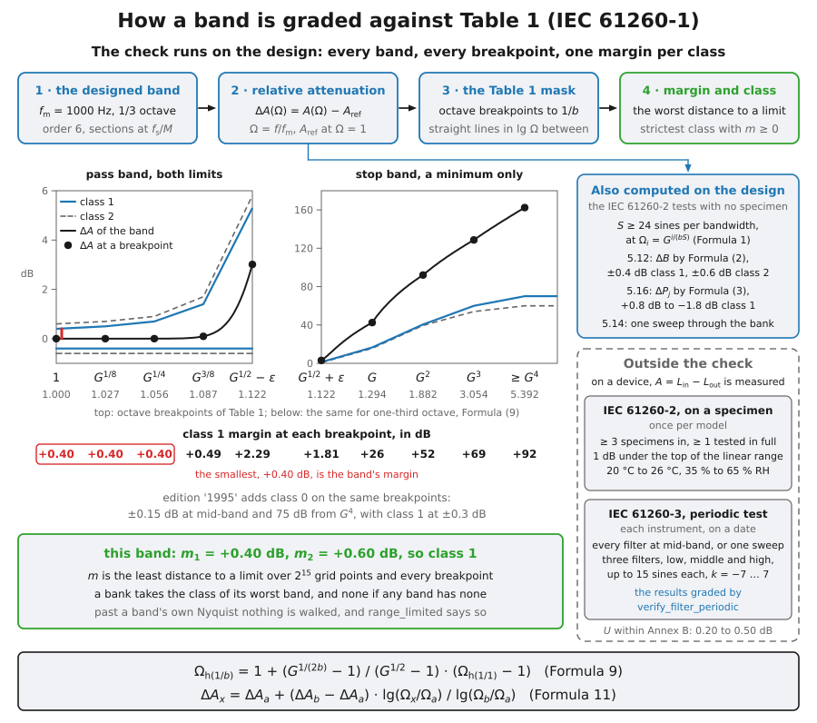
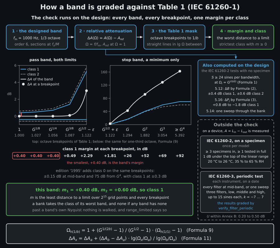
The 1 kHz band of a bank like the one above, walked through the check: its relative attenuation at every Table 1 breakpoint, carried to one-third octave, against the class 1 and class 2 limits, with the smallest margin deciding the class. The default bank walks it to the end of the mask: its Nyquist frequency at 48 kHz is 24 times its mid-band frequency, and a decimated band keeps its own at least sixteen times its upper edge. The box on the right is what section 1b computes on the design as well, the IEC 61260-2 tests that need no specimen; the dashed column under it is what a laboratory does to an instrument, and section 3b grades the periodic-test results it returns.
How far up the mask the verdict actually reaches. checked_to_omega is the
highest normalized frequency at which that band was evaluated:
the band’s own processing Nyquist frequency, which on a multirate bank is the
Nyquist frequency of its decimated rate. The bank decimates a band only as far
as that Nyquist frequency stays at least sixteen times its upper band edge
(section 1b says why), so every decimated band of the bank above is evaluated
to or more, past the end of the Table 1 mask (at least
70 dB for class 1 from up, the octave row carried
to one-third octave). The bands that stop short are the ones filtered at the
full rate near the top of the bank: from 5 kHz up the 24 kHz Nyquist frequency
lies below , and the 20 kHz band is evaluated only to
. There the far-stopband requirement is not demonstrated on
the band filter at all. It is taken as satisfied because a sampled signal
carries no energy above its Nyquist frequency: the anti-alias filter of the
capture chain removed it before the band ever saw it. range_limited is the
flag that this argument was used, and it is True here.
Say that plainly in a report: the verdict attests the mask up to
checked_to_omega, and the rest is an argument about the capture chain. The
flag clears only when every band’s Nyquist frequency lies past the end of the
mask. The one-third-octave bank of section 1b, from 125 Hz to 4 kHz at
48 kHz, is not range-limited; the octave bank over the same range is, because
its 2 kHz and 4 kHz bands, filtered at the full rate, are evaluated only to
and 6, short of the where the octave mask
ends. When a document requires the full mask on every band filter, lower the
top of the bank or raise fs: designing the bank with
design=filters.FilterDesign(resample=False) changes nothing here, because
the bands that stop short already run at the full rate.
What the margin measures. It is the minimum, over every normalized frequency
the band was evaluated at, of the distance to the nearest limit of that class:
positive when the response stays inside the corridor everywhere, and negative by
exactly the worst violation when it does not. The reported class is the
strictest class for which that margin and the margins of section 1b are all
non-negative.
Which constraint binds is worth knowing before you try to improve the number. A
maximally-flat Butterworth is flat at mid-band, where the class 1 corridor is
±0.4 dB, so its margin saturates at +0.400 dB the moment the stopband stops
being the limiting factor: measured on a 48 kHz one-third-octave bank, order 2
fails outright (class None, worst class 1 margin −27.03 dB) and orders 4, 6, 8
and 10 all hold exactly +0.400 dB on Table 1 (order 4 then misses class 1 on
the summation of section 1b, and orders 6 to 10 are class 1 throughout). Raising the order therefore
helps only while the margin is negative for a stopband reason; once a design
passes, the margin is capped by the passband half-corridor and no order will
move it. A margin of +0.400 dB is not a mediocre result to be improved; it is
the best a compliant design can report against this mask.
The Table 1 acceptance mask itself is public too: class_limits(fraction, filter_class, omega) returns the minimum/maximum relative-attenuation
limits at normalized frequencies , the same limits the
verifier and the figure below use.
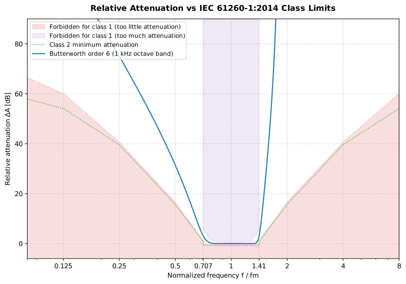
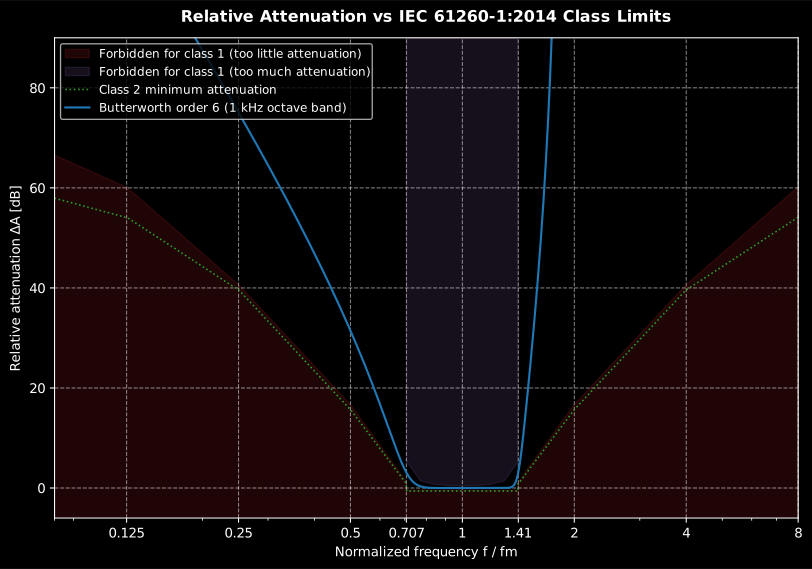
The order-6 Butterworth response (blue) threads between the forbidden regions: it must attenuate at least the red mask outside the band and no more than the purple mask inside it.
Show the code for this figure
import matplotlib.pyplot as pltimport numpy as npfrom scipy.signal import sosfreqzfrom phonometry import filters
fs = 48000bank = filters.OctaveFilterBank(fs, fraction=1, order=6, limits=[800, 1200])idx = int(np.argmin(np.abs(np.array(bank.freq) - 1000)))fm, fsd = bank.freq[idx], fs / bank.factor[idx]w, h = sosfreqz(bank.sos[idx], worN=2**15, fs=fsd)att = -20 * np.log10(np.abs(h) + 1e-12)delta_a = att - np.interp(fm, w, att)     # relative attenuation
grid = np.logspace(np.log10(0.05), np.log10(8), 2000)lo1, hi1 = filters.class_limits(1.0, 1, grid)     # class 1 min/max attenuation
fig, ax = plt.subplots(figsize=(9, 5.5))ax.fill_between(grid, -10, lo1, alpha=0.15, color="tab:red",                label="Forbidden: too little attenuation")finite = np.isfinite(hi1)ax.fill_between(grid[finite], hi1[finite], 90, alpha=0.15, color="tab:purple",                label="Forbidden: too much attenuation")ax.plot(w / fm, delta_a, label="Butterworth order 6")ax.set(xscale="log", xlim=(0.08, 8), ylim=(-6, 90),       xlabel="Normalized frequency f / fm",       ylabel="Relative attenuation [dB]")ax.legend()plt.show()
With default parameters (order 6), Butterworth meets the class 1 mask of
Table 1, and so does Chebyshev II: its attenuation default is now 72 dB, clearing the 70 dB
far-stopband class 1 limit (scipy pins the cheby2 equiripple floor at exactly
attenuation, so any value qualifies; the 72 dB default
keeps the same +0.400 dB passband margin as Butterworth). Chebyshev I,
Elliptic and Bessel do
not meet class limits at order 6: passband ripple (cheby1/ellip) and slow
roll-off (bessel) violate the mask. Class 1 is the strictest verdict this
edition can return; the stricter class 0 the default bank also clears belongs to
the withdrawn 1995 mask and is section 2. Whether a whole bank is class 1 also
depends on the two requirements of section 1b, and the default octave and
one-third-octave banks meet class 1 there too.
1b. Effective bandwidth and the summation of outputs (IEC 61260-2)
Section titled “1b. Effective bandwidth and the summation of outputs (IEC 61260-2)”Table 1 judges a band one frequency at a time. IEC 61260-1:2014 adds two
requirements that judge a band, and a set of bands, as a whole, and
IEC 61260-2:2016 says how a pattern-evaluation laboratory computes them from
the same relative attenuation. Neither needs anything but the designed
response, so for the 2014 edition verify_filter_class grades both, and a
band’s class is the strictest class it meets on all three.
Effective bandwidth (5.12). For broadband sound a band analyser reports the power its band lets through, so its width in power is what matters. The normalized effective bandwidth is Formula (13) of IEC 61260-1,
and its deviation from the bandwidth of an ideal band, , is , within ±0.4 dB for class 1 and ±0.6 dB for class 2 (5.12.2). A band with dB reads pink noise 0.05 dB high. The verifier evaluates the integral as IEC 61260-2 7.2.3.2 recommends: the trapezoidal rule of its Formula (2) over the test frequencies of its Formula (1),
with at least 24 frequencies per bandwidth (points_per_bandwidth, 24 by
default), carried out to the outermost breakpoint of Table 1, where a class 1
band is at least 70 dB down.
Summation of output signals (5.16). A tone between two mid-band frequencies has to come out of the set with its power, shared between the bands that see it, neither lost nor added. Formula (3) of IEC 61260-2 sums on an energy basis the relative attenuation of band and of its two neighbours, at the test frequencies inside band ():
and the result has to stay between −1.8 dB and +0.8 dB for class 1, and between
−3.8 dB and +1.8 dB for class 2. The two end bands, with a neighbour on one side
only, are left out (7.2.4.4), so the requirement is graded only on a bank of
three bands or more, and result.requirements says whether it was. The printed
Formula (3) and the words of 7.2.4.3 and of 5.16 take the difference in
opposite directions, which with limits this lopsided is not the same test; the
verifier applies the limits to the formula as printed, as 7.2.4.5 instructs,
and the errata registry records the conflict.
from phonometry import filters
third = filters.verify_filter_class(    filters.OctaveFilterBank(48000, fraction=3, order=6, limits=[125, 4000]))print(third.overall_class)                                  # 1
octave = filters.verify_filter_class(    filters.OctaveFilterBank(48000, fraction=1, order=6, limits=[125, 4000]))print(octave.requirement_class("relative_attenuation"))     # 1print(octave.requirement_class("effective_bandwidth"))      # 1print(octave.requirement_class("summation"))                # 1print(round(octave.binding_margin_db("summation", 1), 2))   # 0.64print(octave.overall_class)                                 # 1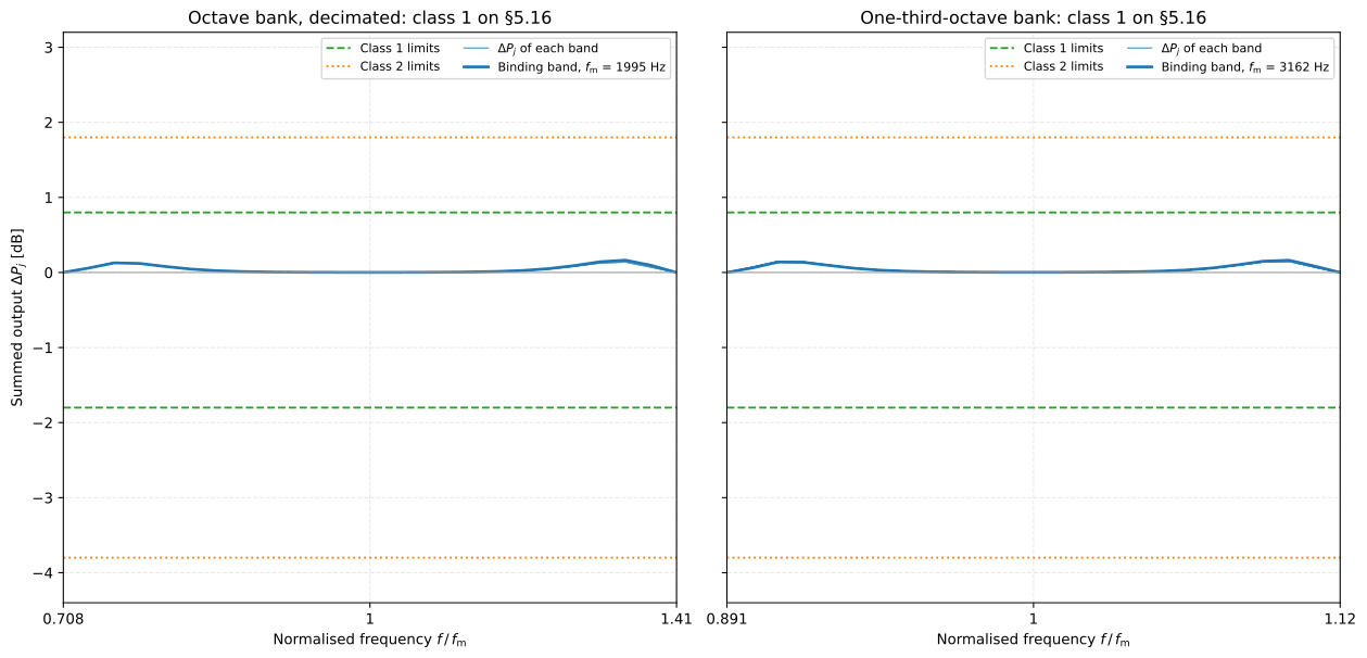
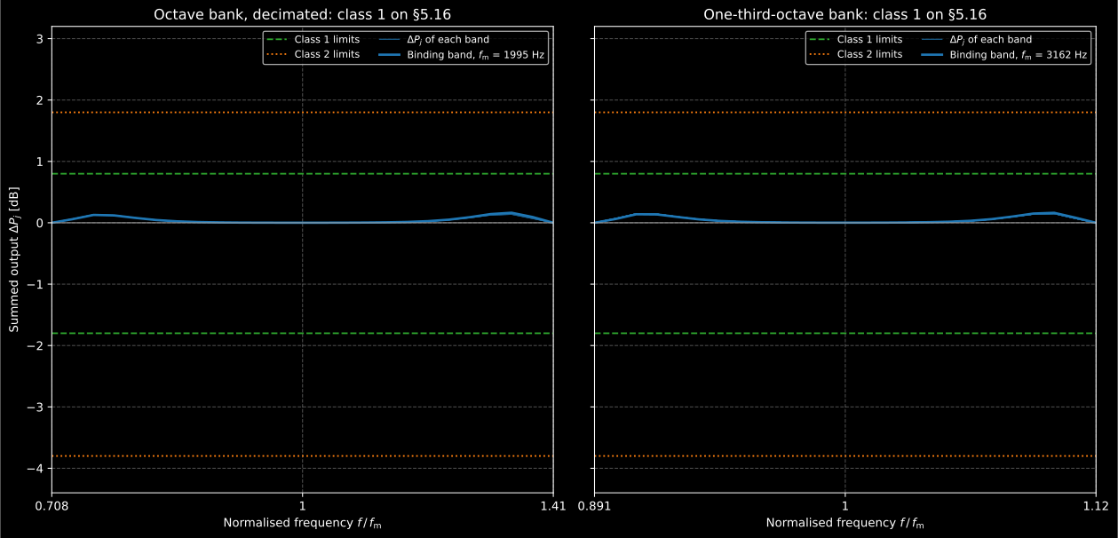
Formula (3) of IEC 61260-2 on every inner band of the two default banks, drawn
by result.plot(requirement="summation"). Both banks return a tone’s power to
within 0.16 dB: the sum stays within a few hundredths of a decibel of 0 dB
across the middle of each band and rises by a little more than a tenth of a
decibel just inside its edges, where two neighbouring bands share the tone.
Show the code for this figure
import matplotlib.pyplot as pltfrom phonometry import filters
octave = filters.verify_filter_class(    filters.OctaveFilterBank(48000, fraction=1, order=6, limits=[125, 4000]))third = filters.verify_filter_class(    filters.OctaveFilterBank(48000, fraction=3, order=6, limits=[125, 4000]))fig, (ax_oct, ax_third) = plt.subplots(1, 2, figsize=(13, 6.2), sharey=True)octave.plot(ax=ax_oct, requirement="summation")third.plot(ax=ax_third, requirement="summation")ax_oct.set_title("Octave bank, decimated: class 1 on §5.16")ax_third.set_title("One-third-octave bank: class 1 on §5.16")ax_third.set_ylabel("")plt.show()
Why the bank decimates a band only to sixteen times its upper edge. The
summation is the requirement a multirate design puts at risk. Close to its own
Nyquist frequency the bilinear transform bends a band: just inside its upper
band edge it attenuates less than the same band designed far from Nyquist, and
above that edge it falls more steeply. Just below an upper band edge the band
and its neighbour above then pass more than the tone’s power; just above a
lower band edge the band below has already fallen away and power is lost. An
octave bank (Butterworth, order 6, 48 kHz) decimated until each band’s
processing Nyquist frequency was only 1.25 times its upper band edge sums its
adjacent outputs from −1.16 dB to +0.94 dB about the input: past the +0.8 dB of
class 1, a class 2 bank. The bend shrinks as the square of that ratio: it moves
the summation of an octave band by 0.074 dB at a ratio of four, 0.018 dB at
eight and 0.005 dB at sixteen, and that of a one-third-octave band by 0.002 dB
at sixteen. So the bank stops decimating a band while its processing Nyquist
frequency is still at least sixteen times its upper band edge, and its
decimated banks sum as the same banks designed at the full rate
(design=filters.FilterDesign(resample=False)): class 1 on every requirement
at 44.1, 48 and 96 kHz. Over its full default range at 48 kHz the octave bank
sums from −0.06 dB to +0.69 dB, decimated or not, the top set by the 8 kHz
band next to the 16 kHz band, which runs at the full rate close to the 24 kHz
Nyquist frequency: class 1 with 0.11 dB to spare. The one-third-octave bank
sums from −0.25 dB to +0.76 dB, both at its 16 kHz band, a margin of 0.04 dB,
and the decimated Chebyshev II octave bank from −0.08 dB to +0.64 dB. None of
this is an artefact of grading transfer functions: tones run through the bank
itself, its decimation filters included, read the Formula (3) sums to within
0.01 dB.
1c. Time-invariant operation (5.14)
Section titled “1c. Time-invariant operation (5.14)”A multirate bank does not filter a tone the same way wherever it falls against the decimation, and a transfer function cannot show that. IEC 61260-1:2014 5.14 tests it on the running filter instead: a sinusoid of constant amplitude whose frequency rises one decade in 2 s to 5 s, and each band’s time-averaged output has to stay within ±0.4 dB (class 1) or ±0.6 dB (class 2) of the level of Formula (17),
the output of an ideal band of the same bandwidth. swept_band_level is that
formula (107.97 dB for the example Annex B of IEC 61260-2 and -3 works
through), and swept_level_uncertainty its standard uncertainty from the
uncertainties of the sweep (Annex A). verify_time_invariance runs the test of
IEC 61260-2 7.4 on a bank: the sweep of Formulas (A.3) and (A.4) goes through
every band exactly as OctaveFilterBank.filter processes a signal, polyphase
decimation included, at 2 s and at 5 s per decade.
from phonometry import filters
bank = filters.OctaveFilterBank(48000, fraction=3, order=6, limits=[25, 10000])swept = filters.verify_time_invariance(bank)print(swept.overall_class)                       # 1print(round(swept.worst_deviation_db, 3))        # 0.056print(swept.seconds_per_decade)                  # (2.0, 5.0)print(round(filters.swept_band_level(    127.0, fraction=3, sweep_duration_s=30, averaging_time_s=30,    start_frequency_hz=0.01, end_frequency_hz=1e6), 2))   # 107.97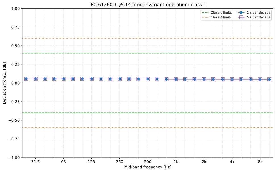
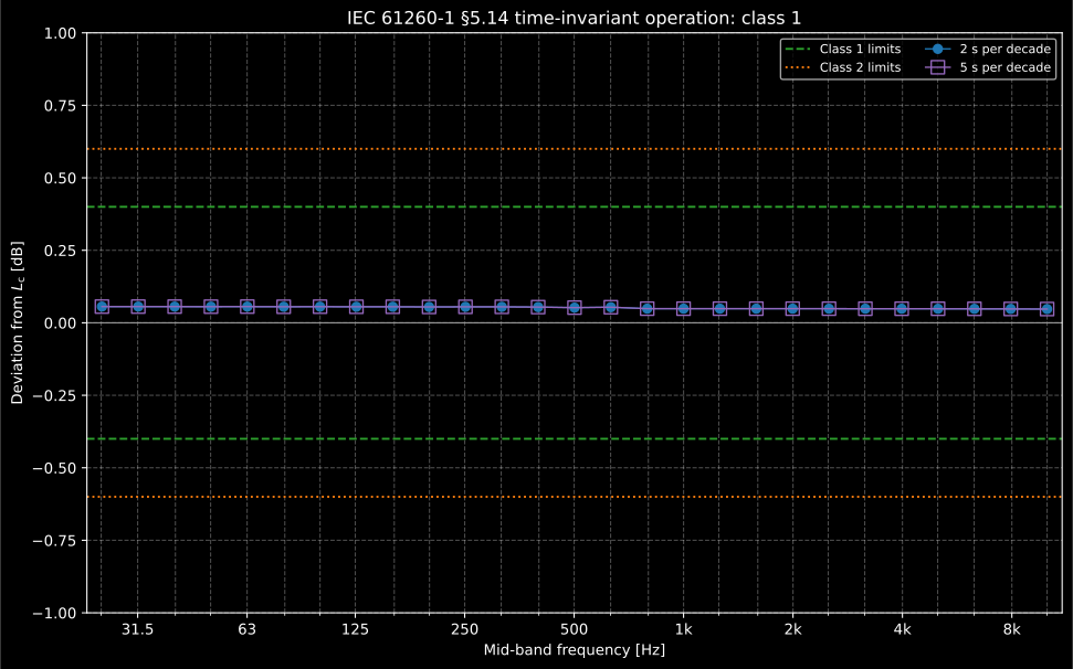
Every band of the decimated one-third-octave bank reads about +0.05 dB at both sweep rates. That is its effective bandwidth deviation of section 1b, which is what Annex G of IEC 61260-1 says a band that behaves as its transfer function must read (G.2.8); decimation that folded energy back into a band would read more, and the two rates would part.
Show the code for this figure
import matplotlib.pyplot as pltfrom phonometry import filters
bank = filters.OctaveFilterBank(48000, fraction=3, order=6, limits=[25, 10000])filters.verify_time_invariance(bank).plot()plt.show()
2. Class 0 (IEC 61260:1995 / ANSI S1.11-2004)
Section titled “2. Class 0 (IEC 61260:1995 / ANSI S1.11-2004)”The tightest performance class, class 0, was defined by the earlier
IEC 61260:1995 and its US twin ANSI S1.11-2004 (both withdrawn/superseded
but still referenced for laboratory-grade instruments); IEC 61260-1:2014 dropped
it. Its class 1/2 masks differ slightly from the 2014 edition, so it lives behind
an edition switch rather than being mixed into the 2014 mask:
from phonometry import filters
fs = 48000bank = filters.OctaveFilterBank(fs, fraction=1, order=6, limits=[800, 1200])
result = filters.verify_filter_class(bank, edition="1995")   # classes 0, 1, 2print(result.overall_class)          # 0  (the default Butterworth clears it)print(result.bands[0]["margin_class0_db"])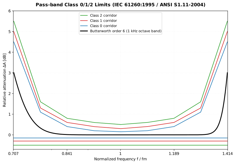
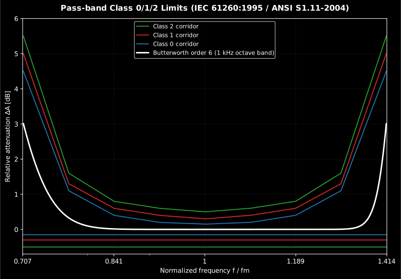
The class 0 corridor (±0.15 dB at mid-band) is the tightest; class 1 (±0.3 dB) and class 2 (±0.5 dB) are progressively wider. The order-6 Butterworth threads inside class 0 across the whole pass-band.
Show the code for this figure
import matplotlib.pyplot as pltimport numpy as npfrom scipy.signal import sosfreqzfrom phonometry import filters
fs = 48000bank = filters.OctaveFilterBank(fs, fraction=1, order=6, limits=[800, 1200])idx = int(np.argmin(np.abs(np.array(bank.freq) - 1000)))fm, fsd = bank.freq[idx], fs / bank.factor[idx]w, h = sosfreqz(bank.sos[idx], worN=2**15, fs=fsd)att = -20 * np.log10(np.abs(h) + 1e-12)delta_a = att - np.interp(fm, w, att)
# Pass-band only: outside the band edges the maximum limit is +inf.g = 10 ** (3 / 10)grid = np.linspace(g ** -0.5, g ** 0.5, 1500)pb = (w / fm >= g ** -0.5) & (w / fm <= g ** 0.5)
fig, ax = plt.subplots(figsize=(9, 5.5))for cls in (2, 1, 0):                      # nested corridors, class 0 tightest    lo, hi = filters.class_limits(1.0, cls, grid, edition="1995")    ax.plot(grid, hi, label=f"Class {cls} corridor")    ax.plot(grid, lo, color=ax.lines[-1].get_color())ax.plot(w[pb] / fm, delta_a[pb], "k", lw=2, label="Butterworth order 6")ax.set(xscale="log", xlim=(g ** -0.5, g ** 0.5), ylim=(-0.7, 6),       xlabel="Normalized frequency f / fm",       ylabel="Relative attenuation [dB]")ax.legend()plt.show()
3. What a class means physically
Section titled “3. What a class means physically”The masks are worst-case error bounds on a measurement, not abstract grades:
-
In the passband the corridor bounds how much the band can mis-read in-band content: a class 1 bank reads a mid-band tone within ±0.4 dB of its true level and a class 2 bank within ±0.6 dB (IEC 61260-1:2014 Table 1; the stricter IEC 61260:1995 Table 1 masks allowed ±0.3 dB for class 1, ±0.5 dB for class 2 and ±0.15 dB for class 0). Toward the band edges the corridor widens, which is the honest admission that a tone sitting exactly on an edge is genuinely ambiguous between two bands (both read it about 3 dB down).
-
In the stopband the minimum-attenuation mask bounds leakage from the rest of the spectrum: far from the band, class 1 demands at least 70 dB of relative attenuation (the reason the
cheby2default is 72 dB). In energy terms, an out-of-band tone must be roughly 70 dB stronger than the band’s own content before it doubles the band’s energy reading (+3 dB). The practical consequence: measuring bands far below a dominant tone, the reading floors out at the leakage skirt about 70 dB down, and a steeper architecture (or higher order) is the only way to push that floor lower.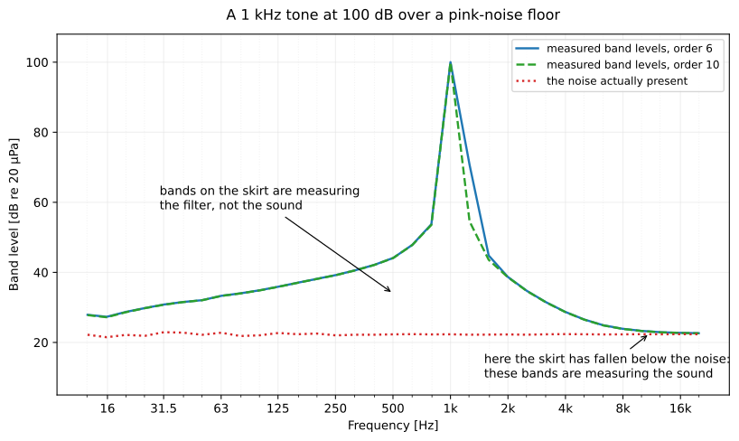
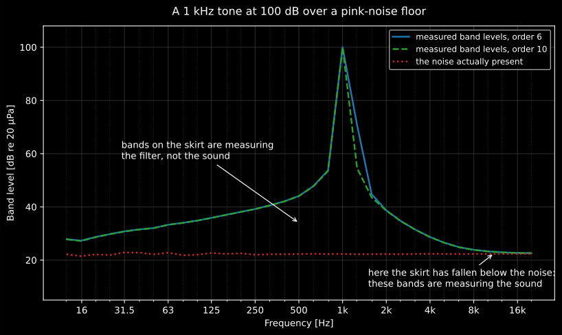
What the last sentence looks like as a measurement. Every band whose level sits on the skirt is reporting the filter’s rejection of the 1 kHz tone, not the sound present in that band: the dotted line is what is really there. The test is not subtle once you look for it: raise the order and the bands that are measuring the filter move, while the bands that are measuring the sound do not.
-
For the uncertainty budget, the class is the filter’s contribution to the measurement uncertainty: a class 1 bank adds up to a few tenths of a dB to a band level, comparable to a class 1 sound level meter’s other tolerance terms, which is why instrument-grade chains specify the class of every stage rather than a single overall figure.
Which architecture reaches which class? Under the 2014 edition, whose only
classes are 1 and 2, the library’s default Butterworth order-6 octave and
one-third-octave banks meet class 1 on every requirement, with a
+0.400 dB margin on Table 1 (the ceiling, and section 1 explains why) and the
summation of section 1b inside class 1 as well. Against the stricter
1995 / ANSI S1.11-2004 mask (edition="1995") the same default reaches
class 0; the configuration the
conformance suite verifies at that class is the octave-band bank at 48 kHz,
so re-run verify_filter_class(bank, edition="1995") yourself before writing
class 0 into a document for any other fraction or sample rate. Writing “class 0
per IEC 61260-1:2014” is a claim against a class that edition does not define.
The table reports the best class each architecture reaches at order 6, fs 48 kHz, under the 1995 mask; the architectures other than Butterworth fall short because they trade the IEC mask for a different property by construction:
| Architecture | Best class (order 6, fs 48 kHz, edition="1995") | Why |
|---|---|---|
butter (default) | 0 | Maximally-flat pass-band, monotone roll-off; fits the mask |
cheby2 | 1 | Flat pass-band but the mask relationship binds at class 1 |
cheby1 | — | Pass-band ripple violates the flatness limit |
ellip | — | Pass- and stop-band ripple |
bessel | — | Flat group delay bought with a slow roll-off |
Under the 2014 edition the same column reads 1, 1 and no class for the other
three: cheby2 joins Butterworth at the top because class 0 no longer exists
to separate them. That is the one-band bank of the figure below; a bank of
several bands adds the summation of section 1b, and the decimated Butterworth
and Chebyshev II octave banks meet class 1 on it too.
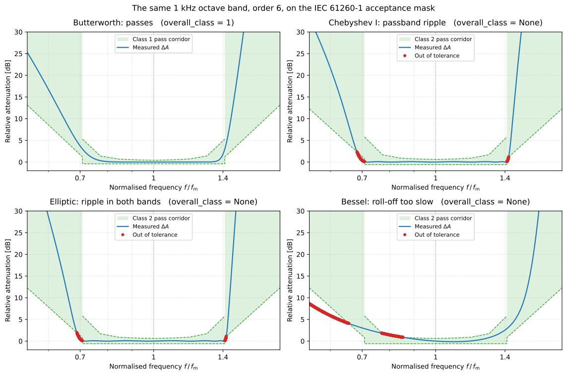
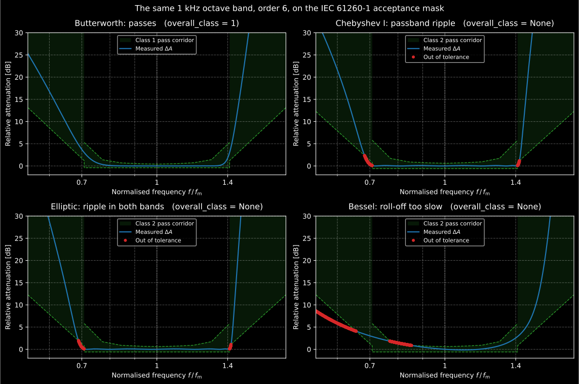
The verdicts of the table, drawn. Chebyshev I and Elliptic poke through the
limit just inside the band edges, where their ripple lives; Bessel leaves it
along the skirt, because it never falls fast enough. The red samples are the
ones verify_filter_class counted against the design, and this is exactly what
verify_filter_class(bank).plot() draws for a bank of your own; note that
the plot shades the corridor of the class each design came closest to, so the
three failing panels show the class 2 corridor.
Show the code for this figure
import matplotlib.pyplot as plt
# `filters` is the import of the snippets above.fs = 48000fig, axes = plt.subplots(2, 2, figsize=(12, 8))for ax, ftype in zip(axes.ravel(), ("butter", "cheby1", "ellip", "bessel")):    bank = filters.OctaveFilterBank(        fs, fraction=1, order=6, limits=[800, 1200],        design=filters.FilterDesign(filter_type=ftype))    result = filters.verify_filter_class(bank)    result.plot(ax=ax)    ax.set_title(f"{ftype}: overall_class = {result.overall_class}")plt.tight_layout()plt.show()
So the sensible default is the common one (Butterworth order 6), while the
alternative architectures are deliberate opt-ins whose purpose (steeper
roll-off, linear phase) works against the class mask. Away from these settings
(very high fraction or near-Nyquist bands), always re-run
verify_filter_class to confirm the class you need.
3b. Verifying an instrument, not a design
Section titled “3b. Verifying an instrument, not a design”verify_filter_class answers a question about a design: does this transfer
function fit the mask. A laboratory answers a different question about a
device on a date, and the two verdicts are not interchangeable.
The full Table 1 walk belongs to pattern evaluation (IEC 61260-2:2016), which a filter-set model passes once, on specimens, under stated climate and after immunity tests. The parts of it that are arithmetic on a response, the effective bandwidth, the summation and the swept test, are sections 1b and 1c; the rest needs the device. What a working instrument actually receives is the periodic test of IEC 61260-3:2016, and it is narrower on purpose: the relative attenuation is measured at the exact midband frequency of every filter in the set, through the electrical input on the reference level range, or, for time-invariant filters, the effective-bandwidth deviation from one exponential sweep across the whole set instead; the relative attenuation of three selected filters, one low, one in the middle and one high, at the clause 13 normalized frequencies ( from to , as far as the frequency range of the set reaches); the linear operating range with its level-range control and overload behaviour; and the lower limit of that range (all under stated environmental conditions and with traceable test equipment). That is why a certificate carries a date, a temperature and a set of serial numbers, and why it says nothing about the parts of the mask it did not walk.
What carries over is worth stating in a report: a class verdict from this page is inherited by every measurement made with the library’s filters, and a hardware chain adds a verdict of its own. Name both. The equivalent regime for sound level meters (IEC 61672-3 periodic tests, and IEC 60942 for the calibrator) is in Calibration and dBFS.
Grading a periodic test. The tests are the laboratory’s to run; the
verdict on what it measured is arithmetic, and verify_filter_periodic does
it. Each result goes in with the laboratory’s expanded uncertainty, and each is
judged by the conformance rule of IEC TC 29 (metrology.verify_conformance):
the deviation within its acceptance limits and the uncertainty within the
maximum IEC 61260-1:2014 Annex B permits for that test. Clause by clause:
| Clause | What the laboratory measured | Acceptance limits | Maximum (Annex B) |
|---|---|---|---|
| 10.2 | relative attenuation of every filter at its exact mid-band | ±0.4 dB class 1, ±0.6 dB class 2 | 0.20 dB, or 0.30 dB past a of 2 dB |
| 10.3 | or, time-invariant filters, from one sweep | ±0.4 dB class 1, ±0.6 dB class 2 | 0.20 dB |
| 11.7 | level linearity on the reference range | ±0.5 dB class 1, ±0.6 dB class 2 within 40 dB of the upper boundary; ±0.7 dB and ±0.9 dB beyond | 0.20 dB within 40 dB, 0.35 dB beyond |
| 11.9 | level linearity on each other range, 30 dB below its upper boundary | as 11.7 | as 11.7 |
| 13 | relative attenuation of three filters at up to 15 | IEC 61260-3 Table 1 | 0.20, 0.30 or 0.50 dB as is up to 2 dB, up to 40 dB, or more |
The fifteen frequencies of clause 13 come from Formulas (1) and (2) of
IEC 61260-3 for any bandwidth designator, periodic_test_frequencies(b), and
its Table 1 is PERIODIC_TEST_ATTENUATION_LIMITS_DB, the stop-band rows with
no maximum. A laboratory drops the frequencies that fall outside the range of
the set (13.4) by writing NaN in their place.
from phonometry import filters
omega = filters.periodic_test_frequencies(3)print(round(float(omega[8]), 5))                          # 1.02667, Table C.1print(filters.PERIODIC_TEST_ATTENUATION_LIMITS_DB[1][7])  # (70.0, inf)
row = [76.0, 63.0, 45.0, 20.0, 0.8, 0.3, 0.1, 0.0, 0.1, 0.2, 0.7, 19.0, 44.0, 63.0, 77.0]row_u = [0.4, 0.4, 0.4, 0.25, 0.15, 0.15, 0.15, 0.15, 0.15, 0.15, 0.15, 0.25, 0.4, 0.4, 0.4]record = filters.FilterPeriodicMeasurements(    midband_attenuations_db=[0.12, -0.05, 0.08, 0.02, -0.1, 0.15],    midband_uncertainties_db=[0.15] * 6,    linearity_deviations_db=[0.0, 0.1, 0.2, -0.3, 0.4],    linearity_levels_below_upper_db=[0.0, 10.0, 20.0, 45.0, 55.0],    linearity_uncertainties_db=[0.12, 0.12, 0.25, 0.2, 0.3],    relative_attenuations_db=[row, [x + 0.2 for x in row], row],    relative_attenuation_uncertainties_db=[row_u, row_u, row_u],)verdict = filters.verify_filter_periodic(1, record, fraction=3)print(verdict.passes)       # Falseprint(verdict.unusable)     # (('11.7', '20 dB below the upper boundary'),)print(verdict.failed)       # ()
Every deviation of that record is inside its limits, and the verdict is still
not a pass: one linearity reading was taken with 0.25 dB of expanded
uncertainty where Annex B allows 0.20 dB, and 5.3 of IEC 61260-3 forbids using
it. verdict.statement says so in the words of the standard, and once every
result is usable it becomes the statement Clause 14 prescribes: 14 k) when the
model’s pattern approval is public (pattern_approval_public=True), 14 l)
otherwise, with the caveat of 1.5 that no general conclusion about
IEC 61260-1 follows from the periodic tests alone.
A pass also needs the tests to cover what the standard asks of them: 11.3 and
13.1 measure three filters, and 13.4 measures each of them at every test
frequency above 0.5 times the lowest mid-band frequency of the set and below
1.5 times the highest. Given the mid-band frequencies of the set
(set_midband_frequencies_hz), of the three tested filters
(tested_midband_frequencies_hz) and of the filter behind each linearity
result (linearity_midband_frequencies_hz), the verdict counts them, and
verdict.incomplete lists each shortfall, a NaN where 13.4 asks for a
measurement included; it holds the pass back as a missing clause does. A
record without them cannot be checked for coverage: verdict.coverage_checked
is False, and a passing statement ends by saying the coverage was not
checked. A mid-band attenuation of 10.2 takes its Annex B maximum from what
was measured, as clause 13 does: a filter that has drifted past 2 dB at its
mid-band is allowed 0.30 dB, and so fails rather than being unusable.
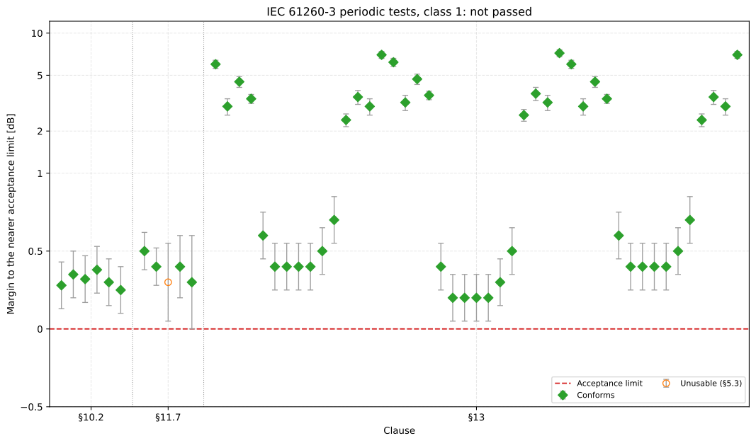
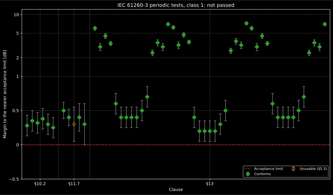
verdict.plot(): every result’s margin to its nearer limit with its expanded
uncertainty, clause by clause. The hollow circle is the one result 5.3 makes
unusable, and it alone holds the verdict back.
Show the code for this figure
import matplotlib.pyplot as plt
# `verdict` is the result of the snippet above.verdict.plot()plt.show()
What the periodic grader leaves to the laboratory report: the self-generated noise of Clause 12, for which Annex B sets no maximum uncertainty, the overload indication of 11.5 and 11.8, and the observations of Clauses 4 and 6 to 8 (preliminary inspection, environmental conditions, the manual) are not graded; record them beside the verdict.
4. The compliance fiche (.report())
Section titled “4. The compliance fiche (.report())”verify_filter_class(bank) returns a result object that exposes .plot()
and .report(), so a type-test verdict can be rendered as a one-page
accredited fiche. The fiche lists every band’s achieved class and
its binding margin over every requirement graded, tabulates the requirements
of sections 1 and 1b with each one’s class, binding margin and range,
overlays the worst-margin band’s measured relative attenuation on the class
corridor, and boxes the overall class-compliance result. Pass a required_class on the ReportMetadata to add a PASS/FAIL
verdict row (a bank “meets class N” when its achieved class is at least as
strict, i.e. a class index of N or lower). The fiche renders in English by
default; pass language="es" for a Spanish fiche (translated fixed strings and
a comma decimal separator), e.g.
result.report("iec61260_es.pdf", language="es").
The example is the decimated octave bank from 125 Hz to 4 kHz, the configuration section 1b shows to be class 1 on every requirement:
from phonometry import ReportMetadata, filters
bank = filters.OctaveFilterBank(fs=48000, fraction=1, order=6, limits=[125, 4000])result = filters.verify_filter_class(bank)   # overall_class == 1result.plot()   # the worst-margin band on its class corridor
result.report(    "iec61260.pdf",    metadata=ReportMetadata(        specimen="1/1-octave filter bank",        measurement_standard="IEC 61260-1:2014",        required_class=1,                # class 1 (or stricter) required    ),)                                        # -> Class 1 - COMPLIES, PASS
The example fiche is regenerated with make reports and kept rendered in the
repository; click the preview to open the PDF.
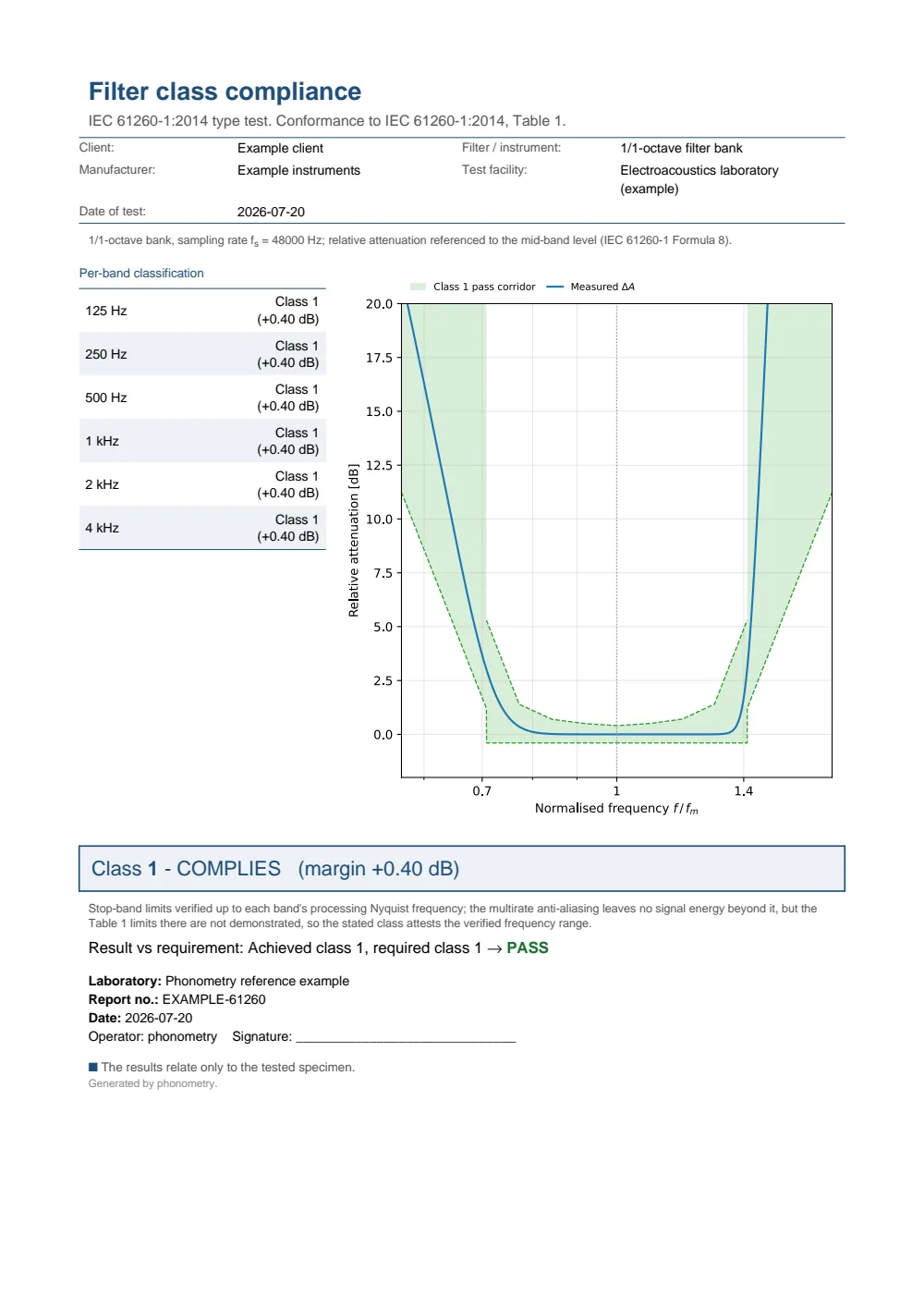
One-page filter-class-compliance fiche: a metadata header, a per-band classification table listing each octave band's achieved class and binding margin, the worst-margin band's measured relative attenuation overlaid on the green class-1 acceptance corridor with the three requirements graded beneath it, the boxed Class 1 - COMPLIES result and a PASS verdict against the required class 1.
Passing edition="1995" verifies against the older IEC 61260:1995 /
ANSI S1.11-2004 mask, which keeps the stricter class 0 that the 2014 edition
dropped, so a modest order-6 bank can be certified to class 0:
bank = filters.OctaveFilterBank(fs=48000, fraction=1, order=6, limits=[250, 4000])result = filters.verify_filter_class(bank, edition="1995") # overall_class == 0result.plot() # the class-0 corridor of the 1995 editionresult.report("iec61260_1995.pdf", metadata=ReportMetadata(measurement_standard="IEC 61260:1995", required_class=0)) # -> Class 0 - COMPLIES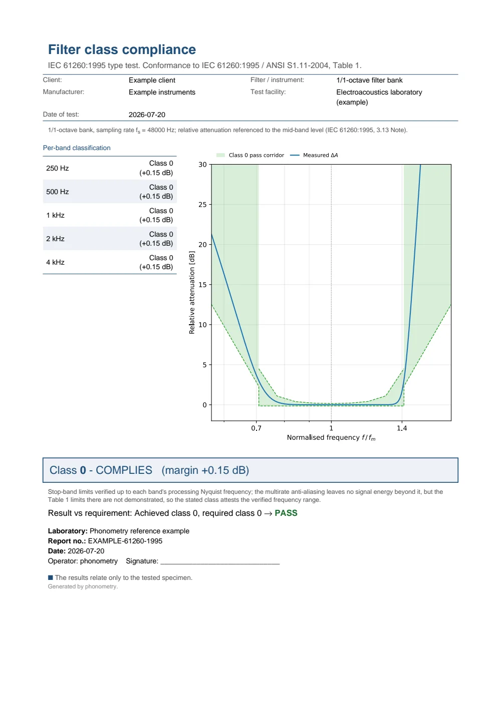
One-page filter-class-compliance fiche under the 1995 edition: a per-band classification table showing every octave band achieving class 0, the measured relative attenuation overlaid on the green class-0 acceptance corridor, the boxed Class 0 - COMPLIES (margin +0.15 dB) result and a PASS verdict against the required class 0.
What this guide covers
Section titled “What this guide covers”Covered
The IEC 61260-1:2014 Table 1 class 1 / class 2 acceptance limits (with the fractional-octave breakpoint mapping and the log-frequency interpolation of the standard), checked band by band by
verify_filter_classand published as a mask byclass_limits; the effective bandwidth deviation (5.12) and the summation of output signals (5.16), graded by the same call as IEC 61260-2:2016 computes them (Formulas (1) to (3)); the swept test of time-invariant operation (5.14, IEC 61260-2 7.4) run on the bank byverify_time_invariance, with Formula (17) and its Annex A uncertainty; the withdrawn IEC 61260:1995 / ANSI S1.11-2004 class 0 mask, reachable withedition="1995"; the grading of a laboratory’s IEC 61260-3:2016 periodic-test results clause by clause byverify_filter_periodic, with its test frequencies, its Table 1 and the statement of Clause 14; and the accredited one-page fiche ofverify_filter_class().report(), with its optionalrequired_classPASS/FAIL verdict, in English and Spanish.Not covered
The tests themselves on a physical filter: the specimens, climate, immunity, overload and linearity tests of IEC 61260-2 and the measurements of IEC 61260-3 are a laboratory’s to run, and
verify_filter_periodicgrades the numbers it returns without producing them. Of those, the self-generated noise of IEC 61260-3 Clause 12 and the overload indications of 11.5 and 11.8 are not graded. Anedition="1995"verdict is its Table 1 mask alone: the effective bandwidth and other requirements of that edition are not graded. Near Nyquist, the bilinear transform warps the frequency axis and the bank has no correction for it, so the stopband mask beyond the processing Nyquist is reported asrange_limitedrather than verified: keep the top band edge comfortably below Nyquist or raisefs.
Quick answers
Section titled “Quick answers”Which filter architecture meets IEC 61260-1 class 1 with default settings?
Section titled “Which filter architecture meets IEC 61260-1 class 1 with default settings?”With the default order 6, Butterworth meets class 1 of the IEC 61260-1:2014
Table 1 acceptance limits, and so does Chebyshev II: its default
attenuation of 72 dB clears the 70 dB far-stopband class 1 limit.
Chebyshev I, Elliptic and Bessel do not: passband ripple (cheby1, ellip)
and slow roll-off (bessel) violate the mask. verify_filter_class reports
the achieved class per band, on Table 1 and on the effective bandwidth and
summation requirements too.
Is the default octave bank class 1 under IEC 61260-1:2014?
Section titled “Is the default octave bank class 1 under IEC 61260-1:2014?”Yes, on every requirement it is graded on: the Table 1 mask, the effective
bandwidth (5.12) and the summation of output signals (5.16). The decimated
Butterworth octave bank sums adjacent outputs within −0.06 dB and +0.69 dB of
the input over its default range at 48 kHz, inside the −1.8 dB and +0.8 dB of
class 1 with 0.11 dB to spare, exactly as the same bank designed at the full
rate with FilterDesign(resample=False): the bank decimates a band only as
far as its processing Nyquist frequency stays at least sixteen times its upper
band edge, where the decimation moves the summation by at most 0.005 dB. The
one-third-octave bank is class 1 on every requirement too, with 0.04 dB to
spare on the summation.
What is class 0 and which standard defines it?
Section titled “What is class 0 and which standard defines it?”Class 0 is the tightest filter performance class, defined by IEC 61260:1995
and its US twin ANSI S1.11-2004 and dropped by IEC 61260-1:2014. Its
passband corridor allows only ±0.15 dB at mid-band, against ±0.3 dB for
class 1 in the 1995 masks. It stays available through edition="1995", and the
default order-6 Butterworth bank meets class 0 in the configuration the
conformance report verifies, the octave-band bank at 48 kHz. Under
IEC 61260-1:2014 that same bank is class 1, on the mask of Table 1 and on
the effective bandwidth and summation of 5.12 and 5.16: the 2014 edition
defines no class 0, so a class 0 claim must cite the 1995 /
ANSI S1.11-2004 mask it was measured against.
References
Section titled “References”- American National Standards Institute. (2004). Specification for octave-band and fractional-octave-band analog and digital filters (ANSI S1.11-2004). Acoustical Society of America. Its Table 1 class limits are identical to those of IEC 61260:1995 and back the same class 0 mask.
- International Electrotechnical Commission. (1995). Electroacoustics — Octave-band and fractional-octave-band filters (IEC 61260:1995). The withdrawn first edition whose Table 1 supplies the stricter class 0 mask offered by edition='1995'.
- International Electrotechnical Commission. (2014). Electroacoustics — Octave-band and fractional-octave-band filters — Part 1: Specifications (IEC 61260-1:2014). The Table 1 class 1 / class 2 acceptance limits verified here, with the fractional-octave breakpoint mapping and the log-frequency interpolation of the standard.
- International Electrotechnical Commission. (2016). Electroacoustics — Octave-band and fractional-octave-band filters — Part 2: Pattern-evaluation tests (IEC 61260-2:2016). The pattern-evaluation regime a filter-set model passes once. Its Formulas (1) to (3), the test frequencies, the trapezoidal effective bandwidth and the summation of adjacent outputs, are how verify_filter_class grades 5.12 and 5.16 of Part 1; its swept test of 7.4, with Annexes A and B, is verify_time_invariance, swept_band_level and swept_level_uncertainty. The specimens, climate, immunity and linearity tests need a physical device.
- International Electrotechnical Commission. (2016). Electroacoustics — Octave-band and fractional-octave-band filters — Part 3: Periodic tests (IEC 61260-3:2016). The periodic tests a working analyser receives: midband relative attenuation of every filter or, for time-invariant filters, the effective-bandwidth deviation from one sweep across the set; the relative attenuation of three selected filters at the clause 13 frequencies; the linear operating range and its lower limit, under stated environmental conditions. verify_filter_periodic grades a laboratory's results against them, with the Formulas (1) and (2) of periodic_test_frequencies and the Table 1 of PERIODIC_TEST_ATTENUATION_LIMITS_DB.