Build a sound level meter

A sound level meter is not one algorithm but a short pipeline of them, and IEC 61672-1 specifies every stage. phonometry implements each stage as an independent, composable function; this page assembles them, in order, into a working meter. Every snippet runs as written (the signals are synthesized so the page is self-contained), and each stage links to the deep guide that explains it fully.

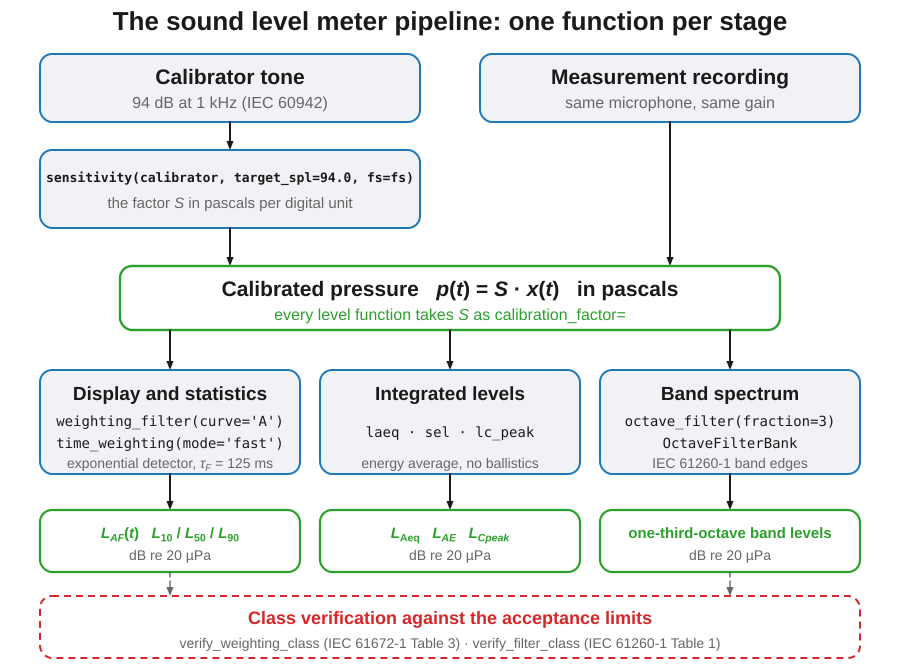
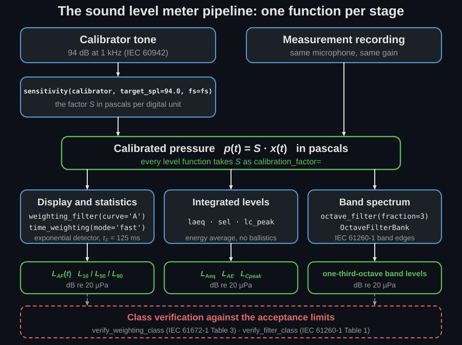
This is the same chain IEC 61672-1 draws for the physical instrument: the class 1 calibrator anchors the microphone to 94 dB at 1 kHz, and every stage that follows is one function of this page.

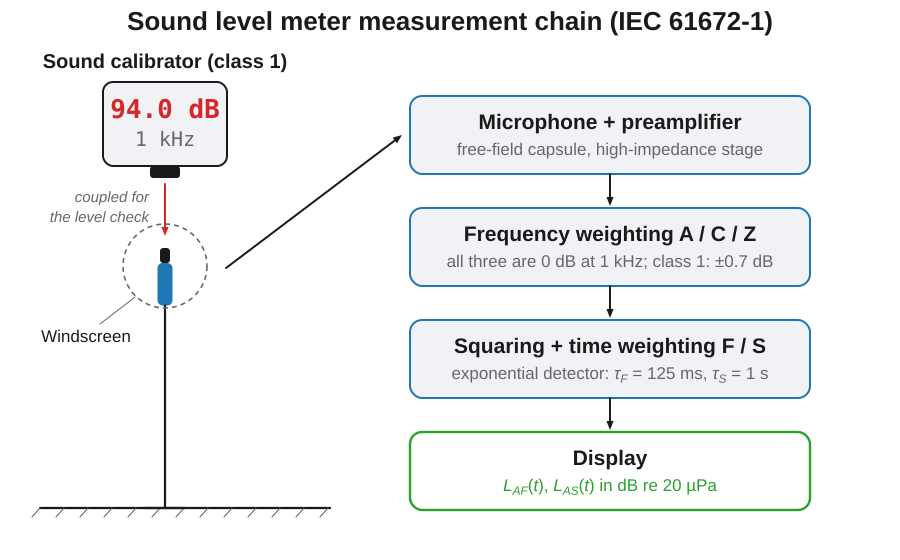
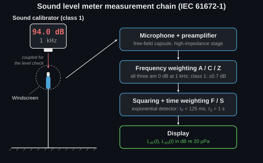
The snippets on this page build on each other: run them top to bottom in one session (or paste the whole page into a script).

1. The scenario

A meter needs two recordings from the same input chain: the calibrator tone that anchors the digital numbers to pascals, and the measurement itself. Here both are synthesized so you can run the page anywhere; in a real measurement they come from your microphone.

import numpy as np
from phonometry import filters, metrology, signals

fs = 48000

# Calibrator tone: 94 dB SPL = 1 Pa RMS at 1 kHz (IEC 60942).
#   Synthesized here; in the field, record a few seconds of your calibrator.
calibrator = np.sqrt(2) * np.sin(2 * np.pi * 1000 * np.arange(3 * fs) / fs)

# "Street" measurement: 10 s of pink background noise plus a 1 s horn-like
#   1 kHz event, so the statistical levels have something to separate.
recording = signals.noise_signal(fs, 10.0, color="pink", rms=0.02, seed=7)
recording[4 * fs : 5 * fs] += 0.2 * np.sqrt(2) * np.sin(
    2 * np.pi * 1000 * np.arange(fs) / fs
)

1b. Recording the two files

A sound level meter built in software inherits every defect of the file it is handed, and three recorder settings decide whether the numbers below mean anything. Set the input gain by hand and lock it. Automatic gain control, limiting and noise suppression all move the sensitivity the next step measures once and step 4 then applies to every sample, so any of them silently voids the calibration. Record uncompressed PCM, 24 bit, at 48 kHz or more. A lossy codec redistributes the high-frequency energy the one-third-octave stage of step 5 reports, and a 44.1 kHz file has no band left above 22 kHz in which to support the class 1 A-weighting of step 3 near 16 kHz. Choose the gain from the loudest event the measurement must be able to prove, leaving roughly 12 dB of headroom above its peak: the $L_{Cpeak}$ of step 4 reads the true inter-sample peak, and one clipped run invalidates it and the $L_{Aeq}$ with it.

Two more decisions belong to the session rather than to the recorder. Record the calibrator tone through that same locked chain immediately before and immediately after the measurement, so the pair brackets the drift that step 7 checks; a factor measured on another day, or after a gain control moved, is not a calibration of this file. Outdoors, keep the windscreen fitted and point the microphone in the reference direction its free-field calibration assumes.

A field sheet worth copying:

• Gain set by hand and written down; AGC, limiter and noise suppression off.
• Uncompressed PCM, 24 bit, $f_s\ge 48$ kHz, one channel per microphone.
• Peak headroom of about 12 dB above the loudest expected event.
• Calibrator tone before and after, same gain, same chain, same session.
• Windscreen fitted, microphone on a tripod, reference direction at the source.
• Sample rate, gain setting, microphone and calibrator identifiers logged.

2. Calibrate: give the samples physical meaning

Digital samples are dimensionless; the sensitivity factor converts them to pascals. sensitivity() computes it from the calibrator recording and, at the same time, validates the recording’s short-term stability the way IEC 60942 qualifies the calibrator itself, so a badly coupled microphone is caught here instead of corrupting every level downstream.

cal = metrology.sensitivity(calibrator, target_spl=94.0, fs=fs)
# cal is in Pa per digital unit; every level function accepts it as
# calibration_factor. For this synthetic tone it is ~1.0.

Deep guide: Calibration and dBFS, which covers the stability check this call runs on the calibrator recording, the integer-format rule, and the digital dBFS mode used when no physical reference exists. With no calibrator at all the factor can be computed from the chain’s rated sensitivity rather than measured — a microphone rated $M$ mV/Pa through a preamplifier of linear gain $G$ into a converter whose full scale is $V_{FS}$ volts gives $S=V_{FS}/(MG/1000)$ pascals per digital unit — but a rated factor carries the datasheet’s tolerance rather than the ±0.4 dB of a class 1 calibrator, so it cannot be reported as a calibrated measurement.

3. Weight: frequency and time (IEC 61672-1)

The meter never shows raw pressure. The signal first passes the A frequency weighting (the ear-response curve of IEC 61672-1), is squared, and is then smoothed by the Fast exponential detector (time constant 125 ms). The result is the moving level a meter’s display follows, $L_{AF}(t)$:

pressure = cal * recording                                # digital units -> Pa
weighted = filters.weighting_filter(pressure, fs, curve="A")
envelope = filters.time_weighting(weighted, fs, mode="fast")  # mean-square Pa^2
laf_t = 10 * np.log10(np.maximum(envelope, 1e-12) / (2e-5) ** 2)
# laf_t peaks near 80 dB during the event and settles near 55 dB between.

A tone burst drives the RC exponential detector: the capacitor charges and drains while the Fast, Slow and Impulse meter needles follow their own ballistics, and the three level traces build up below to show the fast attack, the slow average and the asymmetric impulse hold.

Download the animation (WebM)

A tone burst drives the RC exponential detector: the capacitor charges and drains while the Fast, Slow and Impulse meter needles follow their own ballistics, and the three level traces build up below to show the fast attack, the slow average and the asymmetric impulse hold.

Download the animation (WebM)

The needle in the clip is that time_weighting call: a first-order low-pass charging and draining on the squared signal. The three needles differ in one number, the time constant, which is why Fast catches an event that Slow smooths away. You rarely write this chain yourself: every level function of the next step applies the frequency weighting internally, and the percentile levels rebuild this Fast envelope for you. The energy metrics ($L_{eq}$, SEL) integrate the squared weighted signal directly, with no ballistics at all — which is why they show no needle movement to follow. The chain is shown here because it is the meter’s display.

Deep guides: Frequency Weighting (A, C, Z) and Time Weighting, which takes this same clip apart against the IEC 61672-1 tone-burst table.

4. Integrate: the numbers a meter reports

One pass over the calibrated recording yields the standard readouts: the energy-equivalent $L_{Aeq}$, the percentile levels that describe how the level fluctuated ($L_{90}$ is the background, $L_{10}$ the events), the sound exposure level that normalizes the event to one second, and the C-weighted peak for impulsive content.

la_eq = signals.laeq(recording, fs, calibration_factor=cal)     # ~70.2 dB
ln = signals.ln_levels(
    recording, fs, n=(10, 50, 90), weighting="A", calibration_factor=cal
)                                                # L10 ~78.0, L50 ~55.1, L90 ~54.9
lae = signals.sel(recording, fs, weighting="A", calibration_factor=cal)  # ~80.2
lc_pk = signals.lc_peak(recording, fs, calibration_factor=cal)           # ~84.4

print(f"LAeq {la_eq:.1f} dB | L10 {ln[10]:.1f} | L90 {ln[90]:.1f} "
      f"| LAE {lae:.1f} | LCpeak {lc_pk:.1f}")

Note the arithmetic the numbers encode. The event second measures 80.0 dB on its own and the nine background seconds 55.0 dB, so in energy the event contributes $1\times 10^{8.00}$ and the background $9\times 10^{5.50}=2.9\times 10^6$ — a ratio of about 35:1, or 15.5 dB. The event’s 25 dB head start beats the 9.5 dB ($10{\log }_{10}9$) the background wins back on duration, which is why the 10 s $L_{Aeq}$ of 70.2 dB sits only 0.1 dB above the 70.0 dB the event alone would give spread over the same 10 s: the background is almost invisible in the energy average. $L_{AE}$ is that $L_{Aeq}$ plus $10{\log }_{10}(10\mathrm{s}/1\mathrm{s})=10$ dB, the whole energy compressed into one second. The percentiles read the other way round: the event fills exactly 10 % of the record, so it lifts $L_{10}$ to 78.0 dB and leaves $L_{90}$ at 54.9 dB, the background level.

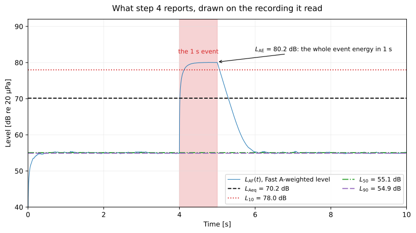
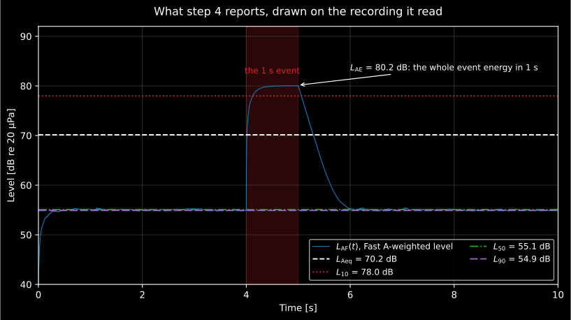
The readouts of this step drawn on the recording that produced them: the event second lifts $L_{Aeq}$ and $L_{10}$, and leaves $L_{50}$ and $L_{90}$ on the background.

Show the code for this figure

import matplotlib.pyplot as plt

t = np.arange(recording.size) / fs
fig, ax = plt.subplots(figsize=(9, 4))
ax.axvspan(4.0, 5.0, color="C1", alpha=0.15)
ax.plot(t, laf_t, linewidth=0.8, label="$L_{AF}(t)$")
for value, name, style in [(la_eq, "LAeq", "--"), (ln[10], "L10", ":"),
                           (ln[50], "L50", "-."), (ln[90], "L90", (0, (5, 1)))]:
    ax.axhline(value, linestyle=style, linewidth=1.0,
               label=f"{name} = {value:.1f} dB")
ax.annotate(f"LAE = {lae:.1f} dB: the whole event energy in 1 s",
            xy=(4.5, lae), xytext=(5.6, lae + 2),
            arrowprops={"arrowstyle": "->"})
ax.set(xlabel="Time [s]", ylabel="Level [dB re 20 µPa]", xlim=(0, 10))
ax.legend(loc="lower right", ncols=2)
plt.show()

Deep guide: Integrated and Statistical Levels, which adds the maximum time-weighted level $L_{AFmax}$ that this same laf_t track yields, noise dose and octave spectrograms; the $L_{den}$ and rating levels continue in Environmental Levels.

5. Band-filter: the spectrum view (IEC 61260-1)

A class 1 meter with a filter set reports band levels. octave_filter decomposes the calibrated signal into fractional-octave bands whose design is anchored to the IEC 61260-1 band edges; nominal=True labels them with the preferred frequencies you would read on an instrument.

spl, bands = filters.octave_filter(
    recording, fs, fraction=3, nominal=True,
    calibration=filters.LevelCalibration(factor=cal),
)
# 33 one-third-octave band levels in dB SPL, labeled '12.5' ... '20k'.
# The '1k' band holds the event: ~70 dB, while its neighbors stay ~25 dB below.
print(dict(zip(bands, np.round(spl, 1))))

These are unweighted (Z) band levels: octave_filter ran on recording, not on the weighted signal of step 3, so their energy sum reproduces the unweighted $L_{eq}$ and not the $L_{Aeq}$ of step 4. That sum is the sanity check worth running once on every measurement:

print(f"sum of the Z bands  {10 * np.log10(np.sum(10 ** (spl / 10))):.1f} dB")
print(f"Leq(Z)              {signals.leq(recording, calibration_factor=cal):.1f} dB")
# sum of the Z bands  70.3 dB
# Leq(Z)              70.4 dB

The tenth or two of deficit is the energy outside the 12.5 Hz–20 kHz analysis range plus the band-edge shapes. A discrepancy larger than about half a decibel points at a calibration or a sample-rate mistake rather than at the filters.

To obtain an A-weighted spectrum, band-filter the already weighted signal of step 3 instead of the raw recording:

spl_a, _ = filters.octave_filter(weighted, fs, fraction=3, nominal=True)
print(f"sum of the A bands  {10 * np.log10(np.sum(10 ** (spl_a / 10))):.1f} dB")
# sum of the A bands  70.2 dB -> the LAeq of step 4, to a hundredth of a decibel

That identity closes the loop between the two halves of the meter: the weighting stage and the filter stage measure the same energy.

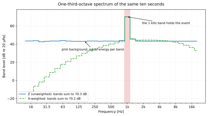
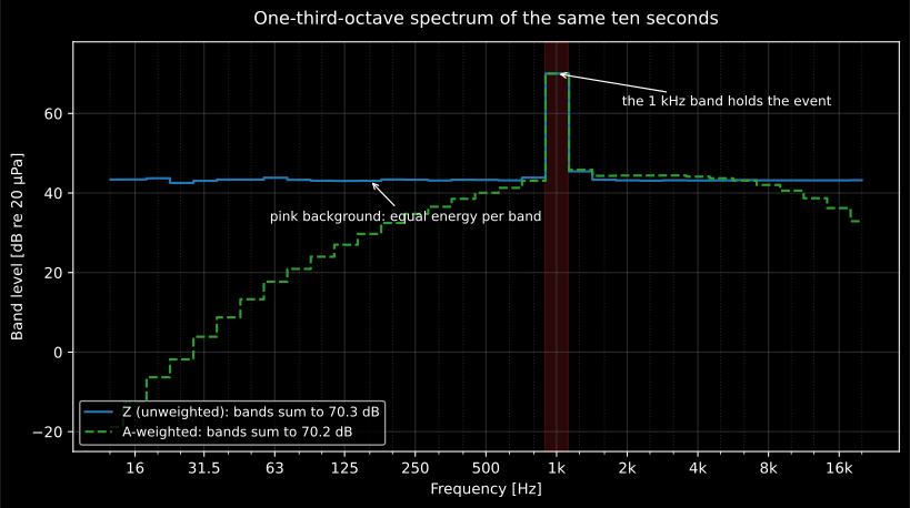
The same recording read in bands, unweighted and A-weighted. Pink noise gives nearly constant fractional-octave band levels, so the flat floor is the background and the single bar 27 dB above it is the event; A-weighting tilts the floor without touching the 1 kHz band, where the A curve is 0 dB.

Show the code for this figure

_, centres = filters.octave_filter(recording, fs, fraction=3)  # exact centres

fig, ax = plt.subplots(figsize=(9, 4))
ax.step(centres, spl, where="mid", label="Z (unweighted)")
ax.step(centres, spl_a, where="mid", linestyle="--", label="A-weighted")
ax.axvspan(891.3, 1122.5, color="C1", alpha=0.15)   # the 1 kHz band
ax.set(xscale="log", xlabel="Band centre frequency [Hz]",
       ylabel="Band level [dB re 20 µPa]")
ax.legend(loc="lower center")
plt.show()

Deep guides: Filter Banks for the filter architectures and zero-phase mode, Block Processing for streaming, and Multichannel and Performance for arrays.

6. Verify: is this meter class 1?

A real instrument is only a “class 1 sound level meter” after its weightings and filters pass the acceptance limits of the standards. The library ships the same verifiers it applies to itself in CI: verify_weighting_class sweeps a WeightingFilter against the IEC 61672-1 Table 3 limits, and verify_filter_class sweeps an OctaveFilterBank against the IEC 61260-1 Table 1 limits.

wf = filters.WeightingFilter(fs, curve="A")
print(filters.verify_weighting_class(wf)["overall_class"])   # 1

bank = filters.OctaveFilterBank(fs, fraction=3)
print(filters.verify_filter_class(bank)["overall_class"])    # 1

The verdicts also come per band, so you can see exactly where a design would leave its class corridor. Deep guides: Frequency Weighting (section on class verification) and Filter Class Verification (the Table 1 mask, class 0 and the compliance fiche).

7. Is this measurement valid?

Step 6 verified the design of the weighting and filter stages. It says nothing about the file. A hardware meter refuses to show a level it cannot stand behind: IEC 61672-1 clause 5.11 makes an overload indicator mandatory (5.11.5 latches it whenever time-averaged or exposure levels are being measured), and clause 5.12 adds an under-range indication. A meter assembled from functions has neither, so three checks on the recording replace them, and each of the three yields a number that belongs in the report.

# (a) Overload: any run of two or more samples pinned at full scale.
at_full_scale = np.flatnonzero(np.abs(recording) >= 1.0 - 1e-6)
runs = (np.split(at_full_scale, np.flatnonzero(np.diff(at_full_scale) > 1) + 1)
        if at_full_scale.size else [])
clipped_runs = sum(1 for run in runs if run.size >= 2)

# (b) Under-range: the same chain capturing its own noise (dummy capsule).
self_noise = signals.noise_signal(fs, 3.0, color="pink", rms=2e-4, seed=11)
margin = la_eq - signals.laeq(self_noise, fs, calibration_factor=cal)

# (c) Drift: the calibrator tone recorded again after the measurement.
calibrator_post = 0.985 * calibrator          # 1.5 % lower in this session
cal_post = metrology.sensitivity(calibrator_post, target_spl=94.0, fs=fs)
drift = abs(20 * np.log10(cal_post / cal))

print(f"clipped runs {clipped_runs} | S/N margin {margin:.1f} dB "
      f"| drift {drift:.2f} dB")
# clipped runs 0 | S/N margin 55.3 dB | drift 0.13 dB

Refuse the record if any clipped run exists, require at least 10 dB of margin over the chain’s self-noise (below that, $L_{90}$ is reading the preamplifier rather than the background), and hold the pre/post sensitivity difference to the 0.5 dB gate of the calibration guide, which also explains why that same difference is the drift term of the uncertainty budget.

Learn the fingerprint of the failure the broadband level hides. Clipping barely moves $L_{Aeq}$ — hard-clipping a 1 kHz tone at 80 % of its peak costs 0.9 dB — while injecting an odd-harmonic ladder that lifts the 3.15 kHz one-third-octave band by 37 dB, the 5 kHz band by 37 dB and the 8 kHz band by 25 dB. A one-third-octave spectrum carrying regularly spaced peaks above anything the source can plausibly radiate is clipping until proven otherwise. The opposite failure looks nothing like it: a signal far below the converter’s range gives a spectrum that barely changes when the source is switched off, which is what check (b) catches.

What this guide covers

• Covered

  This page composes stages already implemented elsewhere into the pipeline IEC 61672-1:2013 describes: the A frequency weighting and Fast exponential time weighting, $L_{Aeq}$, percentile levels, sound exposure level and the C-weighted peak, the IEC 61260-1:2014 octave-band filters of octave_filter, and the Table 3 (weighting) and Table 1 (filter) class acceptance limits checked by verify_weighting_class and verify_filter_class. Each stage’s own guide states its coverage in detail.

• Not covered

  verify_weighting_class and verify_filter_class check the frequency-response design of the digital filters against the standards’ tables; they do not perform the IEC 61672-2:2013 pattern-evaluation tests a physical instrument needs for type approval, such as self-generated noise, linearity range, overload indication or directional response, nor the IEC 61672-3:2013 periodic tests a working instrument receives. A class verdict from this page describes the algorithm, not a built device, and the three checks of step 7 screen the recording, not the instrument. The IEC 60942:2017 calibrator conformance tests are likewise not run here; see the calibration guide for exactly what sensitivity() does and does not check.

See also

The meter built here is the trunk; the rest of the core grows from it.

• Measurement uncertainty (GUM and Monte Carlo): attach an uncertainty to the $L_{Aeq}$ you just computed, calibration term included.
• Calibrated spectral analysis: when bands are too coarse, the Welch PSD with confidence intervals.
• Correlation, time delay and envelope: two microphones instead of one, and the delay between them.
• Block Processing: turn this page’s offline meter into a streaming one with carried filter state.
• API reference: metrology.calibration, filters.weighting, signals.levels, phonometry and filters.compliance.

References

• International Electrotechnical Commission. (2013). Electroacoustics — Sound level meters — Part 1: Specifications (IEC 61672-1:2013). The blueprint of the instrument assembled on this page: the A frequency weighting and the Fast exponential time weighting of the level chain, the C-weighted peak and the sound exposure level, and the Table 3 class acceptance limits checked by verify_weighting_class.
• International Electrotechnical Commission. (2014). Electroacoustics — Octave-band and fractional-octave-band filters — Part 1: Specifications (IEC 61260-1:2014). The fractional-octave-band filters behind the spectrum stage, and the Table 1 class acceptance limits checked by verify_filter_class.
• International Electrotechnical Commission. (2017). Electroacoustics — Sound calibrators (IEC 60942:2017). The acoustic calibrator assumed by the sensitivity stage: the 94 dB principal level and the short-term stability check applied to the reference recording.