Environmental Levels (ISO 1996-1/-2)

A community does not hear a single $L_{Aeq}$: it hears a day whose evenings and nights matter more, a source whose tones or impulses annoy beyond their energy, and a measurement taken over a residual background with a finite confidence. The tonal half of that sentence is this page; the impulsive half belongs to Impulsive sound prominence, which measures the adjustment ISO 1996-1 Table A.1 only tabulates. This page is the regulatory assessment chain built on top of the measured period levels: the whole-day descriptors $L_{den}$/$L_{dn}$ and the composite rating levels of ISO 1996-1, and the ISO 1996-2 determination procedures that make the reported number defensible: the tonal adjustment, the residual-noise correction and the measurement uncertainty budget.

The level computation itself, the $L_{eq}$/$L_{Aeq}$ integrals, the percentile levels $L_N$, SEL and the noise dose that produce the period levels this page consumes, is Integrated and Statistical Levels; everything here assumes those per-period values are already in hand.

Environmental noise: Lden, Ldn and rating levels (ISO 1996-1)

Regulatory noise assessment weights evenings and nights more heavily. lden() implements the day-evening-night level of ISO 1996-1:2016 (3.6.4: +5 dB evening, +10 dB night, default 12/4/8 h periods, adjustable because countries define them differently), ldn() the day-night variant (3.6.5), and composite_rating_level() the general whole-day composite of clause 6.5 (Formulae 5-6) for arbitrary periods with source or character adjustments (Table A.1: e.g. +5 dB regular impulsive, +12 dB highly impulsive, +3 to +6 dB prominent tones):

from phonometry import environment

l = environment.lden(63.2, 58.1, 51.4)                # from LAeq per period
r = environment.composite_rating_level([
    (63.2, 12, 0.0),                                  # day
    (58.1, 4, 5.0),                                   # evening (+5)
    (51.4, 8, 10.0),                                  # night  (+10)
])
print(round(l, 2), round(r, 2))                       # 62.66 62.66

The two agree to the last digit, which is the point of the snippet: lden is composite_rating_level with the three ISO 1996-1 periods and their time-of-day adjustments filled in.

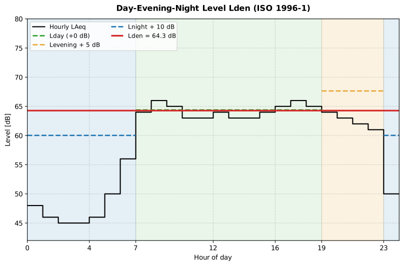
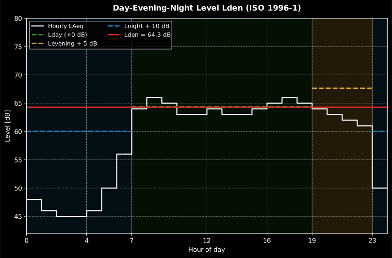
The same day weighted three ways: the evening band is lifted 5 dB and the night band 10 dB before the 12/4/8 h energy average, which is why an $L_{den}$ of 64.3 dB sits above every hourly level of the night.

What 64.3 dB means. The scale is worth carrying: a rural night sits in the 40s, a quiet residential street in the mid-50s, a façade on a busy urban arterial in the high 60s, and the Environmental Noise Directive reports strategic maps in 5 dB $L_{den}$ bands from 55 dB upward. The +5 and +10 dB weights are the price of exposure at the hours when people are at home and asleep, so an evening or a night source moves $L_{den}$ far more than its energy share suggests — in the profile above, the evening is 1.8 dB quieter than the day and lasts a third as long, yet the +5 dB weight gives it 36 % of the energy that makes up the 64.3 dB against the day’s 51 %. Two limits on reading it. The reported indicator is a long-term average: ISO 1996-1 defines its periods over a long-term time interval, normally a year, so the worked day here is one sample of an $L_{den}$ and not an $L_{den}$. And the number is an exposure, not a response; ISO 1996-1 carries annexes that map an adjusted $L_{den}$ or $L_{dn}$ onto an estimated percentage of a population highly annoyed, which is informative and is not implemented here.

Show the code for this figure

import numpy as np
import matplotlib.pyplot as plt
from phonometry import environment

# Synthetic hourly LAeq of an urban road (dB), hours 00 to 23
laeq_h = np.array([48, 46, 45, 45, 46, 50, 56, 64, 66, 65, 63, 63,
                   64, 63, 63, 64, 65, 66, 65, 64, 63, 62, 61, 50], dtype=float)

def period_leq(idx):
    return 10 * np.log10(np.mean(10 ** (laeq_h[idx] / 10)))  # energy mean

ld = period_leq(np.arange(7, 19))                # day 07-19
le = period_leq(np.arange(19, 23))               # evening 19-23
ln_ = period_leq(np.r_[23, np.arange(0, 7)])     # night 23-07
l_den = environment.lden(ld, le, ln_)
print(f"Lden = {l_den:.1f} dB")   # Lden = 64.3 dB

fig, ax = plt.subplots()
ax.axvspan(19, 23, color="C1", alpha=0.15)                                # evening
ax.axvspan(23, 24, color="C0", alpha=0.15); ax.axvspan(0, 7, color="C0", alpha=0.15)
ax.step(np.arange(25), np.r_[laeq_h, laeq_h[-1]], where="post",
        color="0.3", label="Hourly LAeq")
ax.hlines(ld, 7, 19, color="C2", linestyle="--", label="Lday (+0 dB)")
ax.hlines(le + 5, 19, 23, color="C1", linestyle="--", label="Levening + 5 dB")
ax.hlines([ln_ + 10, ln_ + 10], [23, 0], [24, 7], color="C0",
          linestyle="--", label="Lnight + 10 dB")
ax.hlines(l_den, 0, 24, color="C3", linewidth=2, label=f"Lden = {l_den:.1f} dB")
ax.set(xlabel="Hour of day", ylabel="Level [dB]", xlim=(0, 24))
ax.legend(loc="upper left", fontsize=8, ncol=2)
plt.show()

lden() / ldn() / composite_rating_level() parameters

Function	Key parameters	Notes
lden(lday, levening, lnight, hours=(12, 4, 8))	period $L_{Aeq}$ values [dB]; hours must sum to 24	+5 dB evening, +10 dB night (3.6.4)
ldn(lday, lnight, hours=(15, 9))		+10 dB night (3.6.5)
composite_rating_level(periods)	iterable of (level_db, hours, adjustment_db); hours positive, finite and summing to 24	General Formulae (5)-(6); adjustments per Table A.1

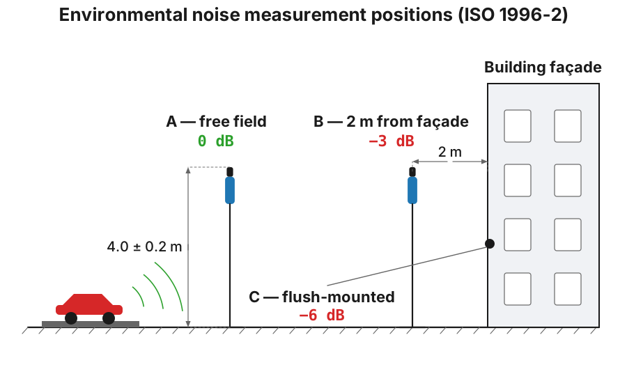
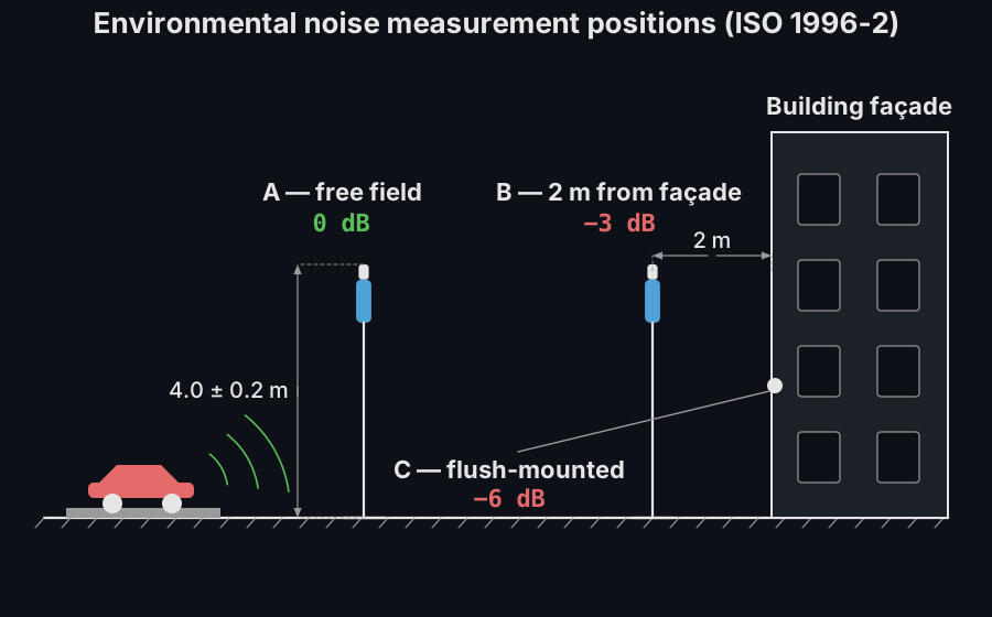
Where you put the microphone changes the number: ISO 1996-2 fixes the receiver positions and their façade corrections. The diagram is measurement context; apply the corrections to your levels before anything on this page:

Microphone location	Correction to reach the incident (free-field) reference	The condition it holds under
Incident sound field	0 dB, this is the reference condition	No reflecting surface other than the ground close enough to matter
Flush-mounted on the façade	Subtract up to 6 dB; exactly 5,7 dB where the Annex B conditions are met	Façade plane within ±0,05 m over 1 m around the microphone, and more than 1 m from any edge of the wall
0,5 m to 2 m in front of the façade	Subtract up to 3 dB; exactly 3 dB where the Annex B conditions are met	An otherwise open situation. Not recommended at near-grazing incidence, and a street canyon or a dense block can make the real difference much larger

(ISO 1996-2:2017, 9.2.1 and Annex B. For general mapping in multi-storey residential areas the same clause fixes the microphone height at (4,0 ± 0,2) m.)

The reason the two corrections are not simply 6 and 3 dB is interference. Flush-mounted, the direct and reflected waves are in phase everywhere on the surface, so the doubling is coherent and broadband — which is why Annex B recommends this position, not the 3 dB one, for stationary sources and low frequencies. Two metres out, the path difference is finite and frequency dependent, so the 3 dB is an ideal-case average that a canyon or a nearby building breaks; Table B.1 puts the standard uncertainty of the correction at 0,4 dB for either position under traffic noise from all angles, but at 2,0 dB for the 5,7 dB position and 1,0 dB for the 3 dB position under predominantly grazing incidence.

Two consequences for everything below. lden, ldn and composite_rating_level consume the corrected level, so applying the correction is the reader’s step and no function on this page will do it. And the reported level must always name its position and state whether a correction was made — a rule the standard states in the same clause, and the reason an END façade indicator, which is defined to include the reflection, must not be corrected at all.

Combine with laeq() per time period to go from recordings to $L_{den}$. The tonal adjustment itself is justified by the tonal audibility route of the next section (fed, for the ISO/PAS 20065 method, by Objective audibility of tones in noise); the tone_to_noise_ratio() / prominence_ratio() verdicts of Prominent Discrete Tones are complementary emission screening, not the $K_t$ basis.

Determining levels: tonal adjustment, residual noise and uncertainty (ISO 1996-2)

ISO 1996-2:2017 is the determination part: how the measured level is turned into a rating level and reported with its uncertainty. The rating-level summation and the time-of-day penalties live in ISO 1996-1 (above); ISO 1996-2 supplies the tonal adjustment, the residual-noise correction and the uncertainty budget.

The measurement behind the numbers (Clause 5)

Everything on this page assumes a level that was obtained the way ISO 1996-2 requires, and the requirements are short enough to state in full.

The whole chain — microphones, cables, windscreens, recording devices and any other accessory — meets class 1 of IEC 61672-1, for free-field or random-incidence application as appropriate, and the filters meet class 1 of IEC 61260 (5.1). A windscreen is always used outdoors, and it does not make wind noise go away: the standard’s own estimate for a 13 mm microphone in a 90 mm windscreen is an A-weighted wind-noise level of about $-18+70{\log }_{10}v$ dB with the wind normal to the diaphragm and $-32+83{\log }_{10}v$ dB with it parallel, $v$ in m/s — which is 31 dB(A) at 5 m/s and 52 dB(A) at 10 m/s, i.e. above the residual of a quiet rural night before the wind is anywhere near a gale. Class 1 tolerance limits themselves only apply between −10 °C and +50 °C.

Calibration (5.2) is a check at the start and the end of every measurement with a class 1 IEC 60942 sound calibrator. The acceptance criterion is explicit: without any readjustment the two consecutive checks must differ by ≤ 0,5 dB, and if they do not, everything measured since the previous satisfactory check is discarded. That is the single rule that most often costs a campaign a day, and it is why the closing check is not optional. For monitoring over several days or more, ISO 20906 takes over.

Verification (5.3) is a valid certificate of compliance against IEC 61672-3, IEC 61260 and IEC 60942, issued by a laboratory meeting ISO/IEC 17025 with traceability to national standards; the recommended interval is once a year and the maximum allowable interval is two years.

The meteorological sensors carry their own maximum permissible errors (5.4), and they are what the uncertainty budget below silently assumes: ±0,5 K for temperature, ±5,0 % for relative humidity, ±0,5 hPa for barometric pressure, ±0,5 m/s for wind speed and ±5° for wind direction.

Finally, a measured environmental level is only reportable with its context. Clause 13 lists what has to be recorded: the time, day and place; the instrumentation and how it was calibrated; the measured and corrected levels; the percentile levels with the base they were computed on; the estimated expanded uncertainty with its coverage probability; the residual sound levels during the measurement; the time intervals; a description of the site including ground cover and the heights of microphone and source above it; and the source operating conditions, including how many events of each category were captured.

Tonal adjustment (engineering method, ISO 1996-2:2007 Annex C)

The 2017 edition dropped the self-contained algorithm and refers to ISO/PAS 20065 instead (Objective audibility of tones in noise); what it keeps is the Annex J table that converts a mean audibility into an integer adjustment. The 2007 algorithm is the one implemented here, because it runs on a single spectrum. From the energy-summed tone level $L_{pt}$ and the masking-noise level $L_{pn}$ in the critical band around a tone, the audibility above the masking threshold is $\Delta L_{ta}=L_{pt}-L_{pn}+2+{\log }_{10}[1+(f_c/502{)}^{2.5}]$ dB (Formula (C.3)), and the adjustment is $K_t=0$ for $\Delta L_{ta}<4$, $K_t=\Delta L_{ta}-4$ for $4\le \Delta L_{ta}\le 10$ and $K_t=6$ above (Formulae (C.4)–(C.6)). The critical bandwidth is 100 Hz up to 500 Hz and 20 % of $f_c$ above (Table C.1). The one-third-octave survey method (tonal_seeking_survey) flags a band exceeding both neighbours by 15/8/5 dB (low/mid/high), and tonal_adjustment_from_mean_audibility maps the ISO/PAS 20065 mean audibility to $K_t$ (Table J.1).

The chain is three functions, not one: tonal_audibility(Lpt, Lpn, fc) returns $\Delta L_{ta}$ from Formula (C.3), tonal_adjustment(dLta) maps it to $K_t$ through Formulae (C.4)-(C.6), and assess_tonal_audibility(...) combines both with critical_bandwidth into the plottable result the snippets below use. The two lower-level functions are the ones the Spanish regulation guide and the wind-turbine guide refer to by name, so they are worth calling directly when only one step is wanted.

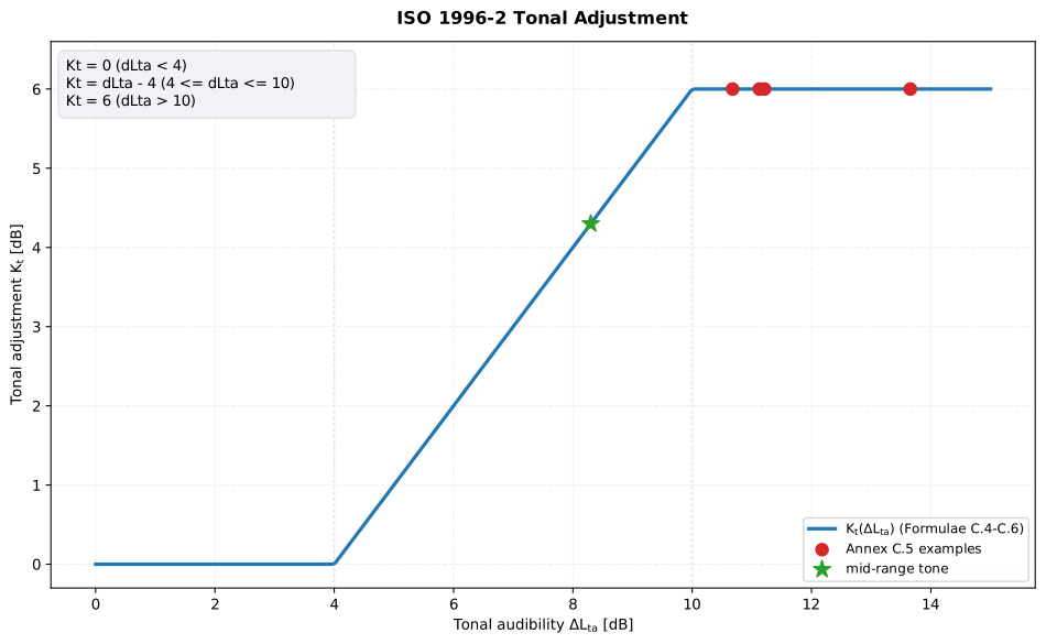
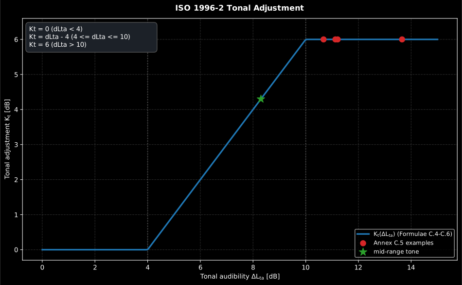
The adjustment saturates at both ends: below 4 dB of audibility a tone costs nothing and above 10 dB it costs no more than 6 dB, so the whole decision lives in a 6 dB window of $\Delta L_{ta}$. All four Annex C.5 examples land in or above that window.

Show the code for this figure

import matplotlib.pyplot as plt
from phonometry import environment

# The worked example is ISO 1996-2:2007 Annex C.5, Example 2 (two tones near
# 400 Hz): the 2017 edition dropped the algorithm and with it its examples,
# so the numbers below come from the edition that carries the method.
# ISO 1996-2:2007 Annex C.5, Example 2 (two tones near 400 Hz):
res = environment.assess_tonal_audibility(tone_level=54.1, masking_noise_level=45.2,
                              centre_frequency=430.0)
print(res.audibility, res.adjustment)   # ΔLta ≈ 11.1 dB -> Kt = 6 dB
res.plot()
plt.show()

Residual-noise correction (Clause 10.4)

residual_sound_correction() applies $L=10{\log }_{10}(10^{L^{\prime }/10}-10^{L_{\text{res}}/10})$ (Formula (16)). With a residual within 3 dB of the measured level no correction is allowed: the uncorrected measured level $L^{\prime }$ is then the reportable value, as an upper bound of the specific sound (exposed as reportable_upper_bound, with reliable=False). gaussian_residual_level() estimates the residual from percentile levels (Annex I) and rejects inverted percentile orderings.

Measurement uncertainty (Clause 4, Annex F)

combined_standard_uncertainty() forms $u=\sqrt{\sum (c_j{u}_j{)}^2}$ (Formula (2)) and expanded_uncertainty() applies $k=2$ (95 %) or $k=1.3$ (80 %); residual_correction_uncertainty() carries the residual-correction sensitivity (Formulae (F.7)/(F.8)) and uncertainty_from_repeated_measurements() the repeated-measurement standard uncertainty: the primary energy-domain route (Formulae (17)+(19)), with the level-domain Note 2 substitute (Formula (20)) reported alongside as approximate_uncertainty and a warning when the levels spread beyond 3 dB, where the substitute grossly inflates.

from phonometry import environment

tonal = environment.assess_tonal_audibility(54.1, 45.2, 430.0)  # TonalAssessmentResult
kt = tonal.adjustment                                             # 6 dB
tonal.plot()   # this audibility on the Kt curve, as in the figure above
corr = environment.residual_sound_correction(measured_level=58.0, residual_level=50.0)

# Table G.2: one hour beside a road under favourable conditions. The five
# contributions are the measured level (0.5 dB scaled by the F.7 sensitivity),
# the source operating conditions (1000 vehicles counted, 10/sqrt(1000)),
# the meteorology, the microphone-location correction and the residual.
u = environment.combined_standard_uncertainty([0.59, 0.3, 2.0, 0.40, 0.38])
print(round(u, 2))                                             # 2.18 dB (G.2)
print(round(environment.expanded_uncertainty(u), 2))           # 4.36 dB (k = 2)

The list is not five anonymous numbers. It is the Table G.2 budget of ISO 1996-2:2017 and every entry has a name, a source and a size:

Contribution	Where it comes from	$c_j{u}_j$
Measured level $L_{eq,1h}$	$u=0,5$ dB — which already absorbs the class 1 sound level meter’s own 0,5 dB default — multiplied by the residual-correction sensitivity $c_{L^{\prime }}$ of Formula (F.7)	0,59 dB
Source operating conditions	1 000 vehicles counted, $10/\sqrt{1000}$ (Formula (8))	0,30 dB
Meteorology	favourable conditions, Formula (12)	2,00 dB
Microphone location	the +5,7 dB flush-mounted correction of Annex B	0,40 dB
Residual sound	$L_{res}=50$ dB with $u=2$ dB, through the sensitivity $c_{res}$ of Formula (F.8)	0,38 dB

combined_standard_uncertainty also accepts $(u_j,c_j)$ pairs, so the sensitivity coefficients need not be pre-multiplied by hand, and residual_correction_uncertainty supplies exactly the two coefficients of Formulae (F.7)/(F.8) — both of which grow without bound as the residual approaches the measured level, which is the same 3 dB cliff as above seen from the uncertainty side.

Now read the column. The meteorology term alone is 2,0 dB and it sets the answer: drop it and the combined uncertainty falls from 2,18 dB to 0,86 dB. The instrument is nowhere near the top of the list. A class 1 meter does not make an environmental measurement accurate — how representative the propagation conditions and the source operation were during that hour is what decides it, and the cheapest way to shrink $u$ is therefore to measure more often, which is what uncertainty_from_repeated_measurements is for.

What this guide covers

• Covered

  ISO 1996-1:2016’s $L_{den}$, $L_{dn}$ and composite rating level (clause 6.5, environment.lden/ldn/composite_rating_level); and ISO 1996-2:2007’s Annex C tonal adjustment together with ISO 1996-2:2017’s residual-noise correction (Clause 10.4), measurement uncertainty budget (Clause 4, Annex F), Annex J mean-audibility mapping and Annex K survey method.

• Not covered

  ISO 1996-2 fixes the receiver positions and the façade corrections that turn a raw measurement into the level this page’s functions expect: those position and correction procedures are not implemented, only the arithmetic that follows once you have applied them.

See also

• Integrated and Statistical Levels: the $L_{eq}$/$L_{Aeq}$, percentile and event levels the indicators of this page are assembled from.
• Impulsive sound prominence (NT ACOU 112): the measured impulsive adjustment $K_I$, and rating_level, which combines impulse-adjusted sub-intervals over a reference time — the sub-daily counterpart of composite_rating_level here, which combines whole periods with their time-of-day and character adjustments (ISO 1996-1 clause 6.5).
• Spanish noise regulation (RD 1367/2007): one national application of exactly this chain, with its own tonal, low-frequency and impulsive corrections.
• Objective audibility of tones in noise (ISO/PAS 20065): the tonal audibility whose mean value maps to the $K_t$ adjustment (Table J.1).
• Prominent Discrete Tones: the ECMA-418-1 tone-to-noise and prominence-ratio verdicts, complementary emission screening for the tonal question.
• Occupational exposure (ISO 9612): the workplace counterpart, from task samples to the daily exposure level with its uncertainty budget.
• API reference: environment.assessment.measurement and environment.assessment.rating.
• Theory: Environmental descriptors (ISO 1996-1): the ISO 1996-1 definitions of the rating level and the day-evening-night indicators, and what the adjustments do to them.

Quick answers

What penalties does Lden apply to evening and night noise?

$L_{den}$, the day-evening-night level of ISO 1996-1:2016 (3.6.4), adds +5 dB to the evening level and +10 dB to the night level before energy-averaging the whole day, with default periods of 12, 4 and 8 hours, adjustable because countries define them differently. The day-night variant $L_{dn}$ (3.6.5) keeps only the +10 dB night penalty.

References

• British Standards Institution. (2003). Description and measurement of environmental noise — Guide to quantities and procedures (BS 7445-1:2003). The survey-practice companion of ISO 1996-1: which descriptor family fits which assessment question, and the measurement procedures around them (BS 7445-2:1991 covers the land-use data acquisition).
• International Organization for Standardization. (2007). Acoustics — Description, measurement and assessment of environmental noise — Part 2: Determination of sound pressure levels (ISO 1996-2:2007). Annex C: the critical bandwidth of Table C.1, the audibility of Formula (C.3) and the piecewise adjustment of Formulae (C.4)-(C.6). This is the self-contained engineering method the library implements; the 2009 corrected reprint is identical here.
• International Organization for Standardization. (2016). Acoustics — Description, measurement and assessment of environmental noise — Part 1: Basic quantities and assessment procedures (ISO 1996-1:2016). Lden (3.6.4), Ldn (3.6.5) and the composite whole-day rating level of clause 6.5 (Formulae 5-6, Table A.1 adjustments).
• International Organization for Standardization. (2017). Acoustics — Description, measurement and assessment of environmental noise — Part 2: Determination of sound pressure levels (ISO 1996-2:2017). The Clause 10.4 residual-noise correction, the Clause 4 / Annex F measurement uncertainty budget, the Annex J Table J.1 mean-audibility mapping and the Annex K survey method.