Spanish Noise Regulation (RD 1367/2007)
Standards: RD 1367/2007Ley 37/2003Key references: Avilés López & Perera Martín 2017
Acoustic assessment in Spain does not stop at an . Real Decreto 1367/2007, which develops Ley 37/2003 del Ruido, defines an index of its own, the corrected equivalent continuous sound pressure level , and builds the whole compliance chain on it: the day is split into evaluation periods, each period into noise phases, each phase is corrected for tonal, low-frequency and impulsive character, the result is integrated up to an annual value, and that value is compared against three different criteria read off the same limit table. This page implements that chain end to end.
The per-period levels that feed it come from Integrated and Statistical Levels, and the European / indicators they coexist with, from Environmental Levels (ISO 1996-1/-2).
The corrected level LKeq and its three corrections
Section titled “The corrected level LKeq and its three corrections”The index of the regulation is (Annex I A.2 c):
where is the A-weighted equivalent continuous sound pressure level,
already corrected for background noise, and the three corrections penalise the
character of the noise. Each is 0, 3 or 6 dB, and their sum is capped at 9 dB
(Annex IV A.3.3), a cap exposed as RD1367_MAX_CORRECTION. Although the index
derives from an A-weighted level, the regulation expresses it in dB.
The background correction every input assumes
Section titled “The background correction every input assumes”above is the level of the activity alone. Everything on this page (the three corrections, the phase levels, the verdict) is defined on a background-corrected level, and the regulation says so before it says anything else. The procedure is the ordinary energy subtraction: measure the residual with the activity stopped, over the same evaluation period, and subtract it from the total, .
It stops being meaningful as the two converge. With the activity 10 dB above the
residual the correction is 0,4 dB and the residual hardly matters; at 3 dB the
correction is 3 dB and the answer is as uncertain as the two measurements that
made it. ISO 1996-2 draws the line there and so should an inspection report: with
a margin below 3 dB no correction is allowed and the honest statement is the
uncorrected level as an upper bound. residual_sound_correction() and the
percentile-based gaussian_residual_level() on
Environmental noise levels
do the arithmetic and carry that rule (reportable_upper_bound,
reliable=False); the RD’s own Annex IV procedure for the measurement series
(how many measurements, how long, what invalidates them) is not implemented here.
Two field consequences. The residual has to be captured in the same evaluation period, because a night residual is not a day residual. And a phase whose margin is too small cannot carry a , or verdict either: all three are differences of background-corrected levels, so the same margin governs the character corrections and not only the level.
| Correction | Input quantity | Thresholds | Function |
|---|---|---|---|
| , emergent tonal components | Unweighted one-third-octave spectrum; , with the arithmetic mean of the two adjacent bands | 8/12 dB (20 to 125 Hz), 5/8 dB (160 to 400 Hz), 3/5 dB (500 Hz to 10 kHz) | tonal_correction() |
| , low-frequency components | 0 dB up to 10 dB, 3 dB for , 6 dB above | low_frequency_correction() | |
| , impulsive components | the same 10 and 15 dB | impulsive_correction() |
is evaluated band by band and, when several emergent tones are present, the largest of the resulting governs (step d):
from phonometry import environment
freqs = [100, 125, 160, 200, 250, 315, 400, 500, 630, 800, 1000]levels = [58.0, 60.0, 59.0, 61.0, 72.0, 62.0, 60.0, 58.0, 56.0, 54.0, 52.0]
kt = environment.tonal_correction(levels, freqs)kt.correction              # 6 dBkt.governing_frequency     # 250.0 Hzkt.differences[4]          # Lt = 10.5 dB above the mean of the neighbours
environment.low_frequency_correction(lceq=76.0, laeq=63.0)   # Lf = 13 dB -> Kf = 3 dBenvironment.impulsive_correction(laieq=68.0, laeq=63.0)      # Li = 5 dB  -> Ki = 0 dBenvironment.corrected_level(63.0, kt=6, kf=3, ki=0)          # LKeq = 72.0 dBenvironment.total_correction(kt=6, kf=6, ki=3)               # 9.0 dB: the cap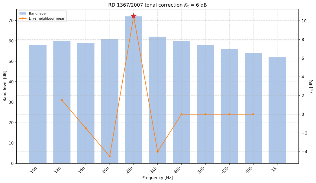
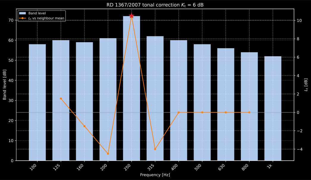
The test is a band against the arithmetic mean of its two neighbours, not against a fitted floor and not against the whole spectrum. Only the 250 Hz band clears its threshold, by 10.5 dB against the 5 dB and 8 dB pair that applies in the 160 Hz to 400 Hz range, so it governs and dB. The two edge bands have no difference at all, because a neighbour is missing.
Show the code for this figure
import matplotlib.pyplot as plt
# `environment`, `freqs` and `levels` come from the snippet above.environment.tonal_correction(levels, freqs).plot()plt.show()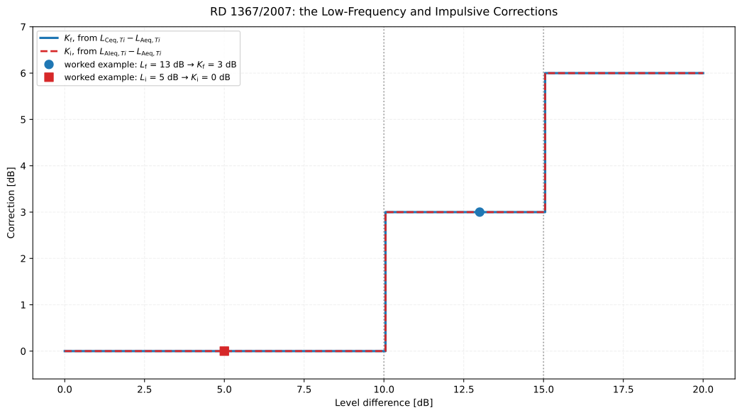
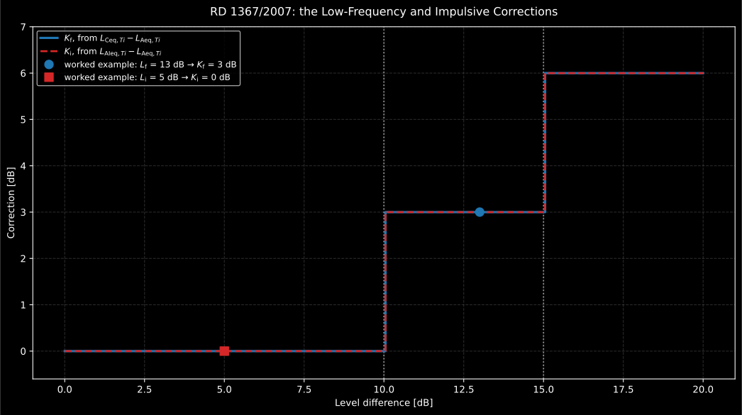
and are the same two-step ladder read off two different meter differences, and the steps are where the arithmetic gets brittle: a difference of 15.0 dB scores 3 dB and one of 15.1 dB scores 6 dB, so a tenth of a decibel of measurement uncertainty on either side of a step is worth 3 dB on .
Show the code for this figure
import matplotlib.pyplot as pltimport numpy as np
# `environment` is imported above.diffs = np.linspace(0.0, 20.0, 400)fig, ax = plt.subplots()ax.step(diffs, [environment.low_frequency_correction(lceq=63.0 + d, laeq=63.0)                for d in diffs], where="post", label="Kf (LCeq - LAeq)")ax.step(diffs, [environment.impulsive_correction(laieq=63.0 + d, laeq=63.0)                for d in diffs], where="post", ls="--", label="Ki (LAIeq - LAeq)")ax.plot([13.0], [3.0], "o", label="worked example: Lf = 13 dB")ax.plot([5.0], [0.0], "s", label="worked example: Li = 5 dB")ax.set(xlabel="Level difference [dB]", ylabel="Correction [dB]")ax.legend(fontsize="small")plt.show()
Relationship with the ISO 1996 procedures
Section titled “Relationship with the ISO 1996 procedures”The corrections of the regulation resemble ISO 1996 procedures the library already implements, but they are not interchangeable, which is why this module implements the RD’s own variants instead of delegating to them:
tonal_audibility()/tonal_adjustment()are the engineering method of ISO 1996-2 Annex C, based on the audibility within the critical band around the tone, and return a continuous between 0 and 6 dB. The RD works on one-third-octave band differences and produces only 0, 3 or 6 dB.tonal_seeking_survey()(survey method, ISO 1996-2:2017 Annex K) is the closest relative, because it also splits the spectrum at 125 and 400 Hz, but it requires the band to exceed both neighbours by 15/8/5 dB and only returns a prominence flag; the RD compares against the mean of the neighbours with 8/5/3 dB thresholds and grades the result.impulsive_sound_adjustment()is the onset-rate method of ISO/PAS 1996-3 on a calibrated signal. The RD’s is the classic difference read off a sound level meter, not the same quantity.- has no counterpart in ISO 1996 at all: the difference is specific to the Spanish regulation.
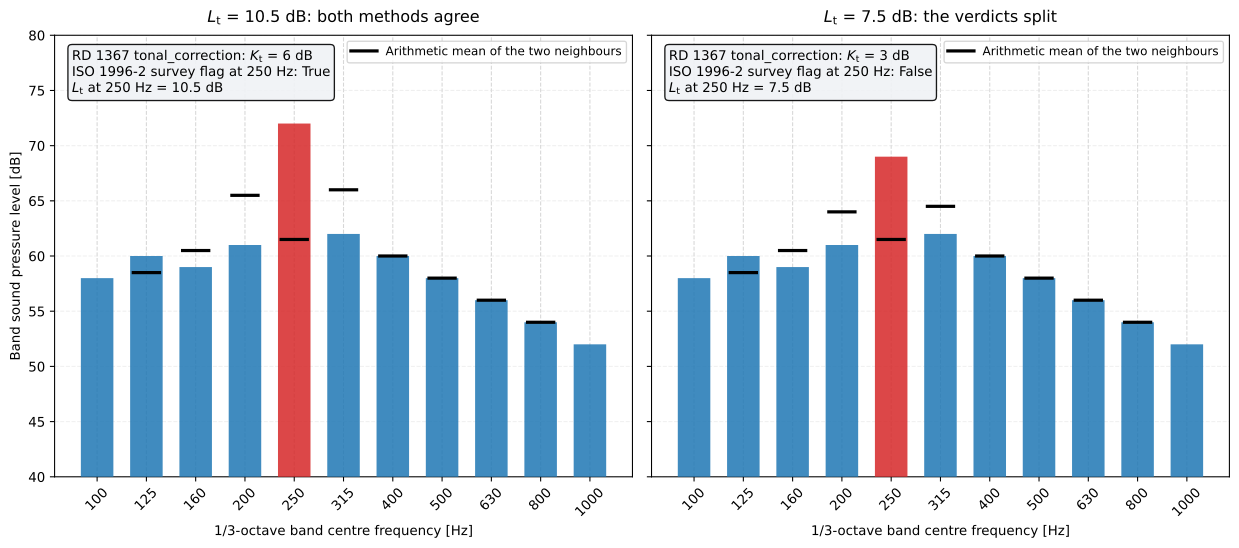
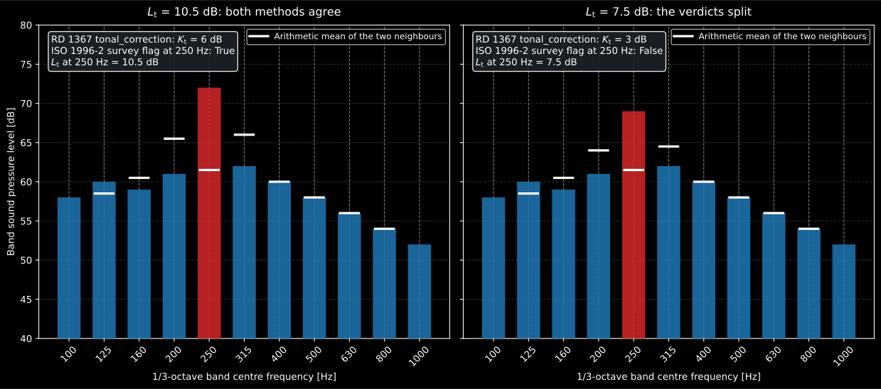
The two procedures are close enough to be confused and far enough apart to disagree on a real spectrum. A 250 Hz band 7.5 dB above the arithmetic mean of its neighbours is graded dB by the regulation and raises no flag at all in the ISO survey method, because it beats each neighbour by less than the 8 dB that method requires. That is exactly the situation an inspection report has to be able to defend: the RD compares against the arithmetic mean of the neighbours with 8/5/3 dB thresholds and grades the result 0/3/6; the survey method requires the band to beat both neighbours by 15/8/5 dB and returns a flag; the Annex C engineering method works inside a critical band and returns a continuous value.
Show the code for this figure
import matplotlib.pyplot as pltimport numpy as np
# `environment`, `freqs` and `levels` come from the corrections snippet above.shallow = list(levels)shallow[4] = 69.0                      # Lt = 7.5 dB instead of 10.5 dB
for spectrum in (levels, shallow):    rd = environment.tonal_correction(spectrum, freqs)    flags = np.asarray(environment.tonal_seeking_survey(spectrum, freqs))    print(rd.correction, rd.governing_frequency, bool(flags[4]))# 6.0 250.0 True     <- both agree# 3.0 250.0 False    <- the RD grades it, the survey method does not flag itplt.show()
Evaluation periods and noise phases
Section titled “Evaluation periods and noise phases”The regulation defines three evaluation periods (Annex I A.1): day from 07:00
to 19:00 (12 h), evening from 19:00 to 23:00 (4 h) and night from 23:00 to
07:00 (8 h), with the durations and clock limits in RD1367_PERIOD_HOURS and
RD1367_PERIOD_CLOCK_LIMITS.
When emission varies within a period, the period is split into noise phases of uniformly perceived level. is measured over at least 5 s in each phase and corrected, and the period level is the energy mean weighted by phase duration (Annex IV A.3.4.2 b):
The annual average of each period is in turn the energy mean of the
daily over the year (Annex I A.2 d). The regulation also fixes its
own rounding: add 0.5 dB to the result and take the integer part, which is what
round_reported_level() does.
from phonometry import environment
environment.RD1367_PERIOD_CLOCK_LIMITS["day"]     # (7, 19)environment.RD1367_PERIOD_HOURS["day"]            # 12.0 h
day = [environment.NoisePhase(2, 0.0, label="cerrada"),       environment.NoisePhase(6, 50.0, kt=6, kf=3),       environment.NoisePhase(4, 48.0, kt=3, kf=3)]
lkeq_d = environment.evaluation_period_level(day)   # 56.82 dB, unroundedenvironment.round_reported_level(lkeq_d)            # 57 dB
lk_d = environment.long_term_corrected_level([57.0, 0.0], weights=[303, 62])environment.round_reported_level(lk_d)              # 56 dB (303 days open, 62 closed)
Acoustic quality objectives and immission limit values
Section titled “Acoustic quality objectives and immission limit values”The regulation separates two families of values. The acoustic quality objectives of Annex II are what the whole set of acoustic emitters reaching an acoustic area or a room must meet; the immission limit values of Annex III are what a single emitter is held to.
| Table | Content | Function |
|---|---|---|
| Annex II, Table A | Outdoor objectives by acoustic area type: e 60/60/50, a 65/65/55, d 70/70/65, c 73/73/63, b 75/75/65 dB (as amended by RD 1038/2012) | outdoor_quality_objectives() |
| Annex II, Table B | Indoor objectives by building use and room type | indoor_quality_objectives() |
| Annex II, Table C | Vibration objective | vibration_quality_objective() |
| Annex III, Tables A1 and A2 | Limit values for new road, rail and airport infrastructure, and | infrastructure_limits(), max_infrastructure_limit() |
| Annex III, Table B1 | Limit values for port infrastructure and activities | activity_limits() |
| Annex III, Table B2 | Noise transmitted by activities to acoustically adjacent premises | adjacent_premises_limits() |
Two details of Table A are worth keeping in mind. Acoustic area type f (general
transport-infrastructure systems and public facilities) carries no numeric
value: footnote 2 refers it to the objectives of the adjoining areas, which is
why ACOUSTIC_AREA_TYPES lists it but the limit functions do not accept it.
And in areas urbanised after the regulation entered into force (24 October
2007) the objective is 5 dB stricter (Article 14.2), which is what
urbanisation="new" applies.
from phonometry import environment
environment.outdoor_quality_objectives("a")                       # 65 / 65 / 55 dBenvironment.outdoor_quality_objectives("a", urbanisation="new")   # 60 / 60 / 50 dBenvironment.indoor_quality_objectives("residential", "bedrooms")  # 40 / 40 / 30 dBenvironment.infrastructure_limits("a")                            # 60 / 60 / 50 dBenvironment.max_infrastructure_limit("a")                         # 85 dB (LAmax)environment.activity_limits("a")                                  # 55 / 55 / 45 dBenvironment.adjacent_premises_limits("residential", "bedrooms")   # 35 / 35 / 25 dBenvironment.vibration_quality_objective("residential")            # 75 dB
Meeting an immission limit value is not simply staying below the number in the table. For activities and port infrastructure, Article 25.1 b) demands three things at once: no annual average above the table value, no daily more than 3 dB above it, and no measured in a noise phase more than 5 dB above it. For the inspection of an activity already in operation, Article 25.2 applies only the last two.
Worked example: a new activity on residential land
Section titled “Worked example: a new activity on residential land”A new activity on residential land (acoustic area type a) opens continuously from 9 to 21 h. A noisy machine runs only between 9 and 15 h; for the rest of the opening hours the levels are steady, and while the activity is shut down it emits nothing. The levels measured outdoors, already corrected for background noise, are:
| Phase | ||||||
|---|---|---|---|---|---|---|
| With the noisy machine | 50 dB | 6 | 3 | 0 | 9 | 59 dB |
| Rest of the opening hours | 48 dB | 3 | 3 | 0 | 6 | 54 dB |
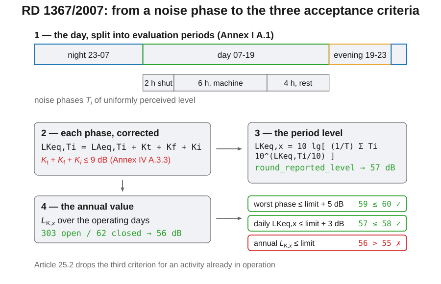
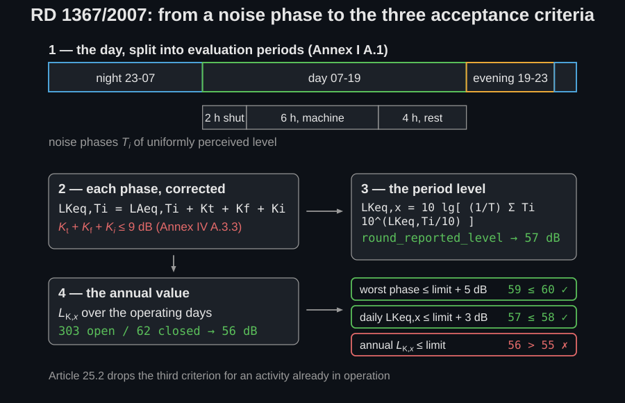
The day period splits into three phases (2 h closed, 6 h with the machine, 4 h with the remaining sources) and gives dB; the evening period splits into two (2 h open, 2 h closed) and gives dB. The activity opens 303 days a year and closes 62 (July and August), from which dB and dB. The limit values for area type a (Annex III, Table B1) are 55/55/45 dB, so the applicable criteria are 60 dB on each , 58 dB on the daily and 55 dB on the annual :
from phonometry import environment
day = [environment.NoisePhase(2, 0.0, label="cerrada"),       environment.NoisePhase(6, 50.0, kt=6, kf=3),       environment.NoisePhase(4, 48.0, kt=3, kf=3)]evening = [environment.NoisePhase(2, 48.0, kt=3, kf=3),           environment.NoisePhase(2, 0.0, label="cerrada")]
limits = environment.activity_limits("a")          # 55 / 55 / 45 dBverdict = environment.assess_activity(    {"day": day, "evening": evening}, limits, operating_days=303)
verdict.periods[0].reported_level        # 57 dB  (LKeq,d)verdict.periods[0].reported_long_term    # 56 dB  (LK,d)verdict.complies                         # False: LK,d exceeds 55 dB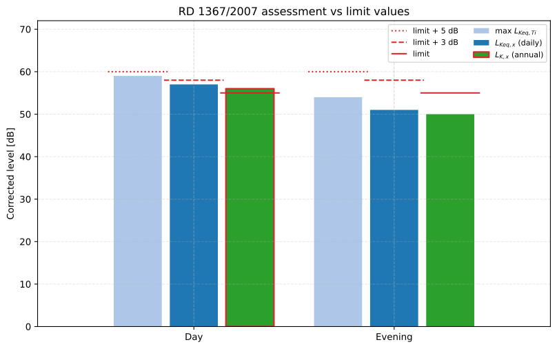
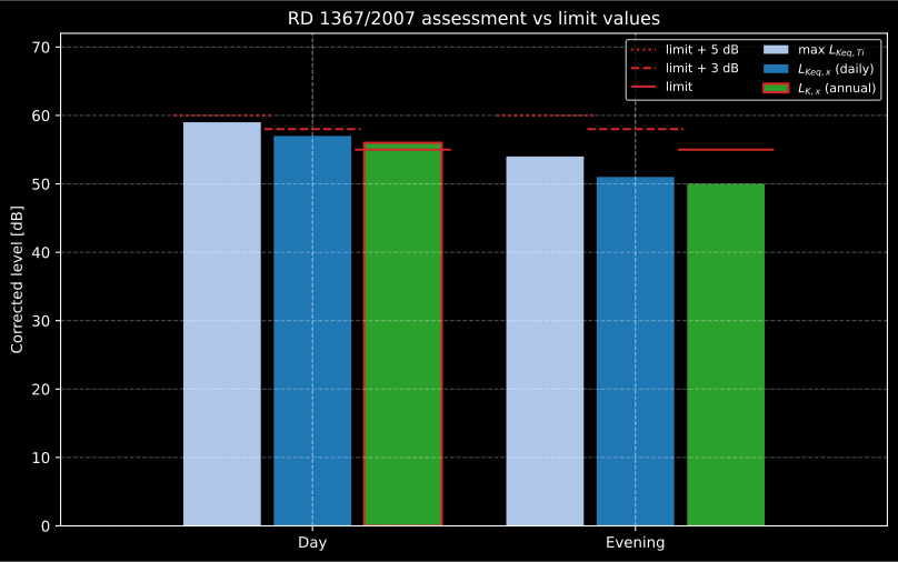
Three indices per period against three different criteria, and only the strictest of them bites. In the day period the worst phase reads 59 dB against its 60 dB criterion and the daily 57 dB against 58 dB (both pass) while the annual of 56 dB fails the 55 dB of Table B1 by one decibel. The evening period (54 / 51 / 50 dB) clears all three. Reading only the loudest bar would declare this activity compliant.
Show the code for this figure
import matplotlib.pyplot as pltfrom phonometry import environment
day = [environment.NoisePhase(2, 0.0, label="cerrada"),       environment.NoisePhase(6, 50.0, kt=6, kf=3),       environment.NoisePhase(4, 48.0, kt=3, kf=3)]evening = [environment.NoisePhase(2, 48.0, kt=3, kf=3),           environment.NoisePhase(2, 0.0, label="cerrada")]
verdict = environment.assess_activity(    {"day": day, "evening": evening},    environment.activity_limits("a"),    operating_days=303,)verdict.plot()plt.show()
The verdict is the fine point of the example. The measured (59 and 54 dB) stay below 60 dB, and the daily values (57 and 51 dB) below 58 dB, but the annual average of the day period, dB, exceeds the 55 dB of the table. A new activity does not comply. An activity already in operation, judged under Article 25.2, would comply, because only the phase and daily values are required of it:
existing = environment.assess_activity( {"day": day, "evening": evening}, limits, operating_days=303, new_activity=False,)print(existing.complies) # True: the annual criterion does not applyPlots and the inspection report
Section titled “Plots and the inspection report”ActivityAssessment.plot() draws the three indices of each period against
their three criteria, as in the figure above, and
TonalCorrectionResult.plot() draws the one-third-octave spectrum with the
differences that justify the applied .
ActivityAssessment.report() goes one step further and renders a one-page
acoustic inspection fiche: identification header, per-phase measurement table
with the // corrections, per-period assessment against the
applicable limit values and the boxed verdict. The default language is Spanish,
the language of the regulation; language="en" translates it.
from phonometry import environment
verdict = environment.assess_activity(    {"day": [environment.NoisePhase(2, 0.0, label="cerrada"),             environment.NoisePhase(6, 50.0, kt=6, kf=3),             environment.NoisePhase(4, 48.0, kt=3, kf=3)],     "evening": [environment.NoisePhase(2, 48.0, kt=3, kf=3),                 environment.NoisePhase(2, 0.0, label="cerrada")]},    environment.activity_limits("a"),    operating_days=303,)
verdict.plot()                       # the three criteria per periodverdict.report("acta.pdf")           # acoustic inspection fiche, in Spanish
The example fiche is regenerated with make reports and kept rendered in the
repository; click the preview to open the PDF.
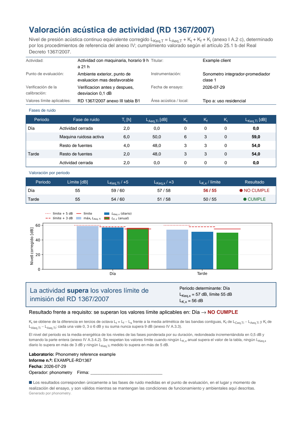
One-page acoustic inspection fiche, rendered in Spanish: an identification header, the noise-phase table of the five phases with their Kt, Kf and Ki corrections and the resulting LKeq,Ti (59,0 dB with the noisy machine running, 54,0 dB for the rest of the sources), the per-period assessment against the 55 dB of Annex III Table B1 (day 59/60, 57/58 and 56/55, evening 54/60, 51/58 and 50/55), the bar plot of each period's levels against its three criteria, and the boxed verdict that the activity exceeds the RD 1367/2007 immission limit values, with the day as the governing period (LKeq,x = 57 dB against a limit of 55 dB, LK,x = 56 dB).
What this guide covers
Section titled “What this guide covers”Covered
The corrected level and the , and corrections of RD 1367/2007 (Annex I A.2 c and Annex IV A.3.3), the evaluation periods and the noise-phase and annual integration (Annex I A.1 and Annex IV A.3.4.2 b) with the regulation’s own rounding, the acoustic quality objective (Annex II) and immission limit value (Annex III) tables, and the Article 25 compliance check of activities and port infrastructure.
Not covered
The acoustic zoning into acoustic areas, the noise maps and the action plans of Ley 37/2003 are planning instruments rather than calculations, and are out of scope. The measurement procedures themselves (microphone positions, series duration, number of measurements of Annex IV) are not implemented either: this page starts where the sound level meter ends.
Quick answers
Section titled “Quick answers”What is the LKeq level of RD 1367/2007?
Section titled “What is the LKeq level of RD 1367/2007?”It is the corrected equivalent continuous sound pressure level: (Annex I A.2 c), where , and penalise the presence of emergent tonal, low-frequency and impulsive components with 0, 3 or 6 dB each. The sum of the three corrections never exceeds 9 dB.
References
Section titled “References”- Avilés López, R., & Perera Martín, R. (2017). Manual de acústica ambiental y arquitectónica. Paraninfo. Ejemplos 3.1 to 3.3 (pp. 171-176) are the worked case reproduced here, with the noise-phase breakdown, the annual integration and the Article 25 verdict. ISBN 978-84-283-3814-1.
- Jefatura del Estado (Spain). (2003). Ley 37/2003, de 17 de noviembre, del Ruido (Ley 37/2003 (BOE-A-2003-20976), consolidated text). The act the RD develops: the acoustic area types of Article 7, the figure of the acoustic emitter and the inspection regime of Articles 25 to 27.
- Ministerio de la Presidencia (Spain). (2007). Real Decreto 1367/2007, developing Ley 37/2003 del Ruido on acoustic zoning, quality objectives and acoustic emissions (RD 1367/2007 (BOE-A-2007-18397), consolidated text). The corrected level LKeq,T and the Kt/Kf/Ki corrections (Annex I A.2 c and Annex IV A.3.3), the evaluation periods (Annex I A.1), the noise-phase integration (Annex IV A.3.4.2 b), the acoustic quality objectives (Annex II) and the immission limit values (Annex III). Table A of Annex II is amended by RD 1038/2012.