Wind-turbine noise: sound power and tonal audibility
Standards: IEC 61400IEC TS 61400ISO 1996
IEC 61400-11 measures the acoustic emission of a wind turbine. This page covers its two closed-form quantities: the apparent sound power level referred to an equivalent point source at the rotor centre, and the tonal audibility that decides whether a discrete tone (blade-passing, gearbox, generator) is audible above the masking noise.
Apparent sound power level
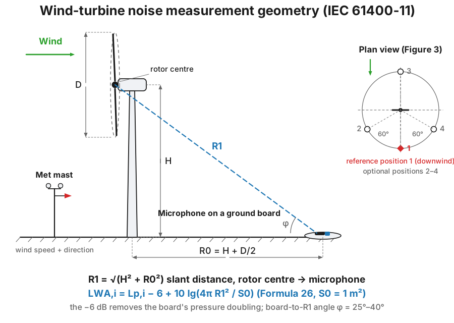
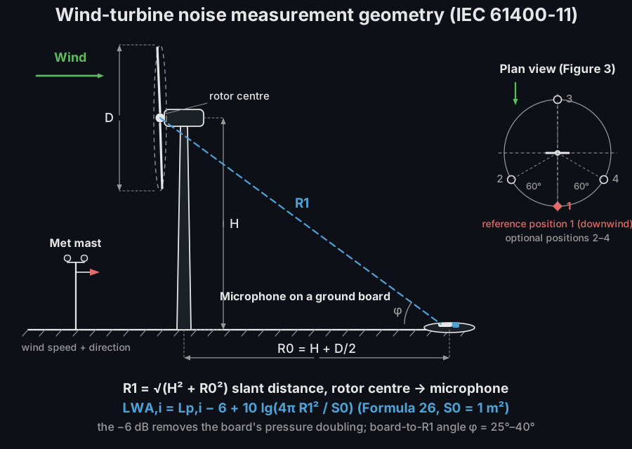
Section titled “Apparent sound power level”With the reference microphone on a ground board at the horizontal distance (hub height , rotor diameter ), the slant distance to the rotor centre is and the apparent sound power level is per band (), energy-summed over bands. The −6 dB accounts for the ground-board pressure doubling.
from phonometry import environment
# Background-corrected A-weighted one-third-octave band levels L_p,i (dB),# here the 250 Hz to 1 kHz bands of a downwind ground-board measurement.band_levels = [55.0, 58.0, 60.0, 57.0, 54.0]          # 250, 400, 500, 800, 1000 Hzr1 = environment.slant_distance(hub_height=80.0, rotor_diameter_m=100.0)print(round(r1, 2))                                   # 152.64 mlwa = environment.apparent_sound_power_level(band_levels, r1)   # dB re 1 pWprint(round(float(lwa), 2))                           # 112.98 dB(A) re 1 pW
The measurement position in practice
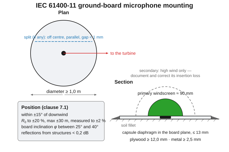
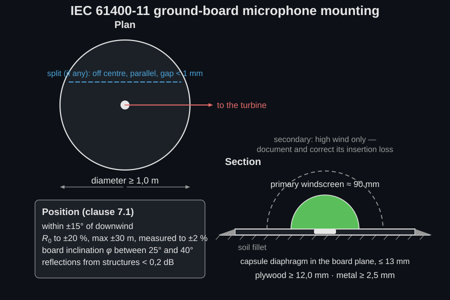
Section titled “The measurement position in practice”The −6 dB above is only the board’s pressure doubling if the board really is a board. IEC 61400-11:2012+A1:2018 fixes what that means, and a tripod microphone or a small plate gives an incoherent reflection instead, which puts the apparent sound power out by an unknown amount rather than a correctable one.
| Requirement | Value | Clause |
|---|---|---|
| Measurement chain | IEC 61672 class 1; filters IEC 61260 class 1; 1/3 octaves from 20 Hz to 10 kHz determined simultaneously; narrowband over 20 Hz to 11 200 Hz | 6.1.2, 6.1.3, 6.1.4 |
| Microphone diaphragm | ≤ 13 mm, in a plane normal to the board, axis pointing at the turbine | 6.1.2, 6.1.5 |
| Board | Circular, diameter ≥ 1,0 m, acoustically hard: plywood or hard chip-board ≥ 12,0 mm, or metal ≥ 2,5 mm | 6.1.5 |
| A split board | Pieces level in one plane, gap < 1 mm, split off the centre line and parallel to the microphone axis | 6.1.5 |
| Seating | Flat on the ground, edges and gaps underneath levelled out with soil | 7.1 |
| Windscreen | Primary: half an open-cell foam sphere ≈ 90 mm across, centred on the diaphragm. Secondary only where a high wind makes the low-frequency signal-to-noise ratio inadequate, and then its frequency response must be documented and corrected in 1/3-octave bands | 6.1.5, Annex E |
| Direction | Within ±15° of the downwind direction at the time of measurement | 7.1 |
| Distance | to ±20 %, at most ±30 m, measured to ±2 %, and as close to as possible; using the tolerance has to be justified in the report | 7.1 |
| Inclination | between 25° and 40°, adjusting the position inside the tolerances above if necessary | 7.1 |
| Reflections | The calculated influence of any reflecting structure < 0,2 dB | 7.1 |
| Calibration | Class 1 IEC 60942 calibrator on the microphone immediately before and after every session, and again whenever a microphone is disconnected and reconnected | 6.1.6, 7.2.2 |
| Traceable verification | Acoustic calibrator 12 months; microphone, sound level meter, recorder, anemometer, power and temperature transducers 24 months; spectrum analyser 36 months | 6.3 |
The causal chain is worth holding on to. The board is what makes the reflection coherent, so the board decides whether the −6 dB is a constant or a guess; the foam hemisphere is what keeps the wind that drives the emission from also driving the microphone’s own self-noise; and the secondary windscreen is the one piece of the setup that changes the answer without changing the sound, which is why the standard makes its insertion loss a documented, band-by-band correction rather than an accepted loss. One measurement position is required and three more are optional: the reference position is downwind and the others exist to document how the emission varies around the machine, not to be averaged with it.
Why “apparent”
Section titled “Why “apparent””is written like a sound power level, but it is not one in the ISO 3744 sense of sampling the pressure field over an enveloping surface. The standard collapses the whole machine into an equivalent point source at the rotor centre and asks what power that source would need, radiating spherically, to reproduce the measured level at one downwind ground-board position: by definition it is the power “giving the same sound emission in the downwind direction as the wind turbine”. Everything a 150 m rotor does that a point source does not, the vertical and lateral directivity and the blade-passing swish, is folded into the number and evaluated in a single direction; the optional positions 2 to 4 of the plan-view pattern exist precisely to document how the emission varies around the machine. Apparent sound powers of different turbines are comparable because the geometry scales with the machine (, so every rotor is seen under a similar angle), which is the point of the definition, but an fed into an ISO 9613-2 prediction carries its built-in downwind bias with it. The ground board, in turn, is why the formula subtracts 6 dB: a capsule lying on a hard plate receives a perfectly coherent reflection (pressure doubling, dB) instead of the uncontrolled height-dependent interference pattern a tripod microphone would sample (see the image source behind the ground effect).
Wind-speed bins and standardized conditions
Section titled “Wind-speed bins and standardized conditions”A turbine’s noise emission rises with wind speed toward rated power, so a single number would be meaningless without its operating point: IEC 61400-11 reports as a function of wind speed.
How a bin is filled. Sound and wind are logged in synchronized 10 s averages, and every period is sorted into a wind-speed bin 0.5 m/s wide centred on integer and half-integer hub-height wind speeds, with at least 10 periods of total noise and 10 of background (turbine parked) per bin. Within each bin the spectra are averaged, interpolated to the bin centre and background-corrected; a total-minus-background margin of 3 dB or less voids the bin, between 3 and 6 dB flags it with an asterisk.
Where the wind speed comes from. Preferably not from an anemometer at all: it is derived from the measured electric power through the turbine’s power curve (Clause 8.2.1), the most repeatable proxy for the wind the rotor actually sees, with the nacelle anemometer and a met mast as fallbacks. The measured range must at least cover 0.8 to 1.3 times the wind speed at 85 % of maximum power (roughly 6 to 10 m/s at 10 m height for a large machine).
Why the abscissa is reported twice. For comparability with consent conditions and older editions, Formula (29) also maps each result to the wind speed at 10 m height over a reference roughness length m (a logarithmic wind profile), giving at integer 10 m wind speeds regardless of the site’s actual terrain. The library implements the closed-form quantities of this pipeline (slant distance, per-band apparent power, tonal audibility); the binning, averaging and uncertainty machinery operates on whole measurement campaigns and stays out of scope.
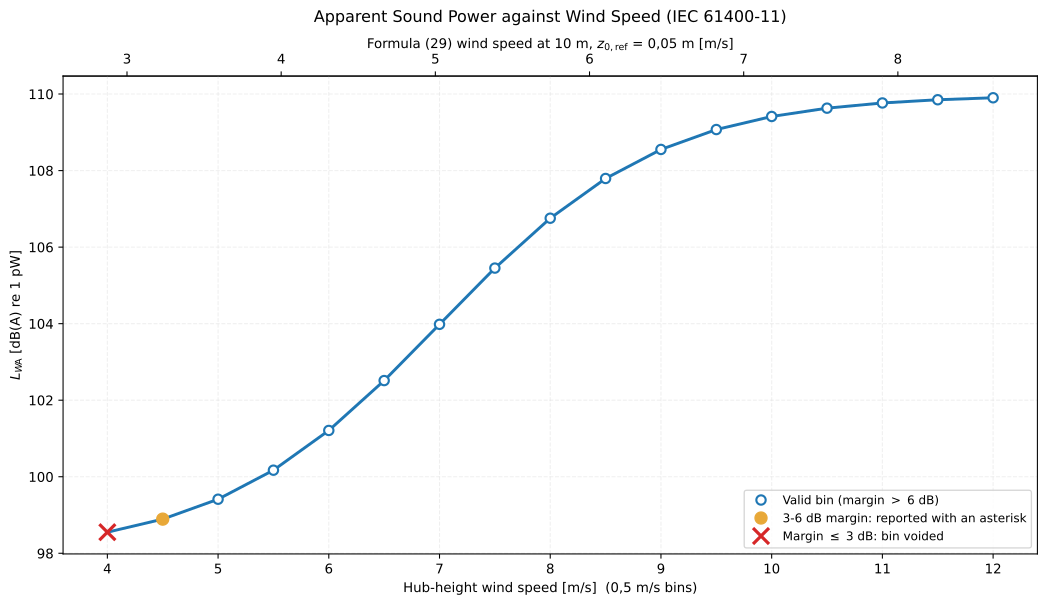
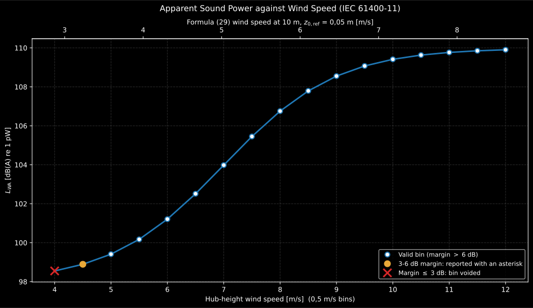
The quantity this standard reports is a curve, not a number: the same machine is 98.6 dB(A) at 4 m/s and 109.9 dB(A) at 12 m/s. The shape is the machine’s control strategy: steepest where the rotor is accelerating, flat once it is at rated power, so quoting a single without its wind speed says nothing. The struck bin and the asterisked one are the standard’s own bookkeeping: below a 3 dB total-minus-background margin the bin is void, between 3 and 6 dB it is reported with a flag. The upper axis is the same series against the Formula (29) 10 m reference wind speed, which is what a consent condition is usually written in and is not the speed the rotor saw.
Show the code for this figure
import matplotlib.pyplot as pltimport numpy as np
# `environment` is imported by the snippet above. The per-bin band levels here# are synthetic: a real campaign supplies them, background-corrected and# interpolated to the bin centre.r1 = environment.slant_distance(hub_height=80.0, rotor_diameter_m=100.0)bins = np.arange(4.0, 12.5, 0.5)shape = np.array([-4.0, -1.5, 0.0, -1.0, -3.0])   # 250 Hz to 1 kHzlwa = [float(environment.apparent_sound_power_level(    44.0 + 12.0 / (1.0 + np.exp(-(v - 7.0))) + shape, r1)) for v in bins]
fig, ax = plt.subplots()ax.plot(bins, lwa, "o-")ax.set_xlabel("Hub-height wind speed [m/s]")ax.set_ylabel("Apparent sound power level LWA [dB(A) re 1 pW]")plt.show()
Tonal audibility
Section titled “Tonal audibility”From a narrowband spectrum (1–2 Hz resolution), the lines in the critical band about the tone, Hz, are classified into masking noise and tone lines (the 70 %-lowest energy mean, the +6 dB criteria; tone lines must additionally lie within 10 dB of the highest line above the threshold, and that highest line is the frequency of the tone, subclauses 9.5.3/9.5.4). The candidate itself must first pass the 9.5.2 possible tone screening: a local maximum more than 6 dB above the band energy average excluding the maximum and its adjacent lines.
For a candidate between 20 and 70 Hz the Zwicker expression is not
meaningful (it is at the bottom of the audible range) and subclause 9.5.3
replaces it with the fixed absolute 20-120 Hz band. The returned
critical_bandwidth is then 100 Hz for every such candidate and the band is
not centred on the tone, which is why a low-frequency
WindTurbineTonalityResult cannot be reconciled with the formula printed above.
For a wind turbine that is not a corner case: blade-passing harmonics and
low-speed gearbox tones live exactly there. The
masking-noise level follows Formula 31, the
tonality is , and the tonal audibility is
with
, reported when
and audible when .
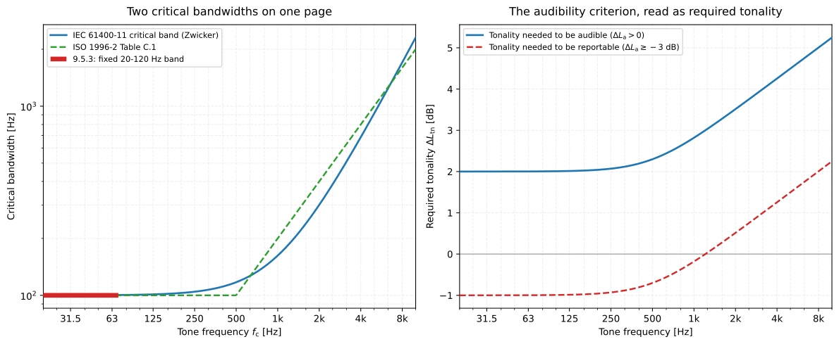
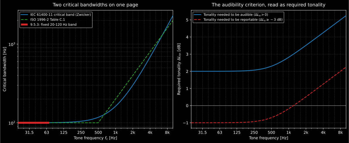
Left: two different critical bandwidths live on this page. The IEC 61400-11
Zwicker band is what WindTurbineTonalityResult.critical_bandwidth reports
(117.3 Hz for the 500 Hz tone of the fiche below), while
environment.critical_bandwidth is the ISO 1996-2 Table C.1 band (100 Hz
up to 500 Hz and 20 % of above it) used by the ISO tonal-audibility
route on the environmental-levels page. They are not interchangeable. Right: the
criterion is nearly flat below 500 Hz and then tightens, so a low-frequency tone
is judged on almost the same emergence as a mid-frequency one; the reportable
line sits 3 dB below the audible one everywhere.
Show the code for this figure
import matplotlib.pyplot as pltimport numpy as np
# `environment` is the module imported by the snippets above.fc = np.geomspace(20.0, 10000.0, 400)zwicker = 25.0 + 75.0 * (1.0 + 1.4 * (fc / 1000.0) ** 2) ** 0.69la = -2.0 - np.log10(1.0 + (fc / 502.0) ** 2.5)
fig, (left, right) = plt.subplots(1, 2, figsize=(12, 4.4))left.loglog(fc, zwicker, label="IEC 61400-11 critical band (Zwicker)")left.loglog(fc, [environment.critical_bandwidth(float(f)) for f in fc], "--",            label="ISO 1996-2 Table C.1")left.plot([20.0, 70.0], [100.0, 100.0], lw=4,          label="9.5.3: fixed 20-120 Hz band")left.set(xlabel="Tone frequency fc [Hz]", ylabel="Critical bandwidth [Hz]")left.legend(fontsize="small")
right.semilogx(fc, -la, label="Tonality needed to be audible")right.semilogx(fc, -la - 3.0, "--", label="Tonality needed to be reportable")right.set(xlabel="Tone frequency [Hz]",          ylabel="Required tonality dLtn [dB]")right.legend(fontsize="small")plt.show()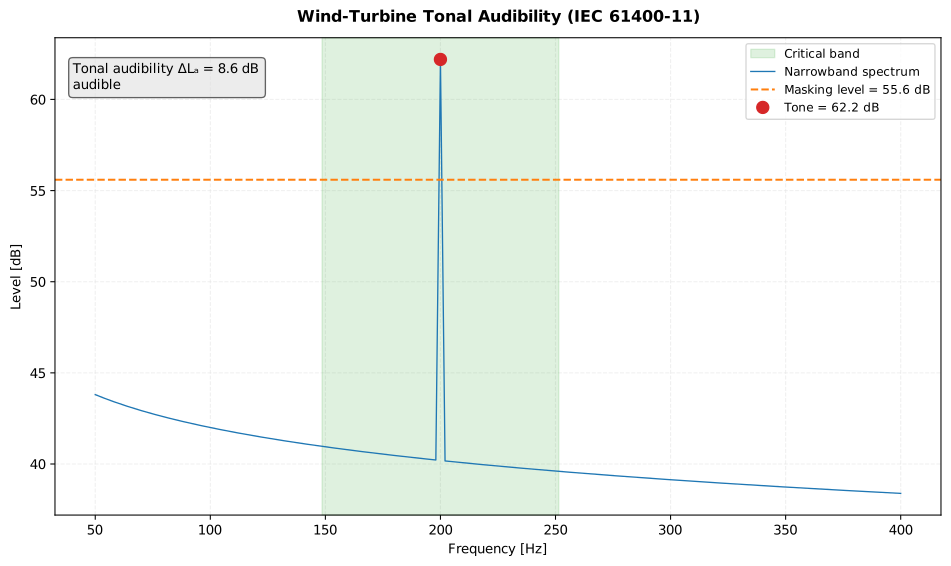
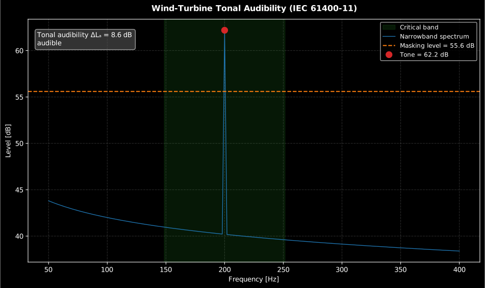
What the method actually compares. The 200 Hz line stands 22 dB above the shaped floor, but the verdict is not that number: inside the 102.9 Hz critical band the classified tone lines sum to = 62.2 dB and the masking noise to = 55.6 dB, so the tonality is 6.6 dB. Only after subtracting the audibility criterion dB at this frequency does the reportable quantity appear, = 8.6 dB, well over the 0 dB that makes the tone audible. The shaded band, not the line height, is what sets it.
Show the code for this figure
import numpy as npfrom phonometry import environment
df = 2.0freqs = np.arange(50.0, 400.0 + df, df)levels = 42.0 - 6.0 * np.log10(freqs / 100.0)levels[int(np.argmin(np.abs(freqs - 200.0)))] += 22.0   # blade-passing-style toneenvironment.wind_turbine_tonality(levels, freqs, tone_frequency=200.0).plot()
import numpy as npfrom phonometry import environment
# A uniformly-spaced narrowband spectrum (2 Hz resolution): a flat 30 dB floor# with a discrete 60 dB tone at 500 Hz.frequencies = np.arange(440.0, 562.0, 2.0)levels = np.full(frequencies.size, 30.0)levels[np.argmin(np.abs(frequencies - 500.0))] = 60.0
res = environment.wind_turbine_tonality(levels, frequencies)print(res.tone_frequency, res.tonality, res.tonal_audibility, res.is_audible)res.plot() # spectrum + critical band + masking level (needs matplotlib)wind_turbine_tonality returns a WindTurbineTonalityResult with the
critical_bandwidth, tone_level, masking_level, tonality,
audibility_criterion, tonal_audibility, is_audible and
has_identified_tone. When the candidate fails the 9.5.2 screening or no
line classifies as “tone”, has_identified_tone is False: the numeric
fields are non-standard fallbacks and such spectra must be excluded from
the 9.5.1 energy averaging of over the spectra of a wind-speed bin
(is_audible also requires an identified tone). The tone frequency and the
criterion anchor to the highest classified tone line, not the probed
candidate. The audibility formula coincides with ISO 1996-2 Annex C; what is
specific to IEC 61400-11 is the determination of the tone and masking levels
and the Zwicker critical band from the spectrum. IEC 61400-11 stops at
and prescribes no adjustment, so which mapping gives the rating
adjustment depends on the edition the assessment is made under. The
9.5.1 energy average over the spectra of a wind-speed bin is a mean
audibility, which is the quantity ISO 1996-2:2017 Table J.1 was written for:
tonal_adjustment_from_mean_audibility,
integer 0-6 dB (or coarse=True for the 0/3/6 ladder of its note). The
piecewise (C.4)-(C.6) law of tonal_adjustment is the 2007 Annex C mapping and
applies to one spectrum’s , and the two differ by 1 to 2 dB on
the same input: dB gives by Table J.1 and 1.0 dB by
Annex C, dB gives 4 dB and 5.0 dB. The notation differs too:
this page’s is that page’s , and the two printings
carry the criterion with opposite signs.
Assessment report (.report())
Section titled “Assessment report (.report())”WindTurbineTonalityResult.report(path) renders a one-page PDF fiche laid out
like the tonality assessment of an environmental-noise laboratory, following
IEC 61400-11:2012+A1:2018 (subclauses 9.5.2 to 9.5.8): a standard-basis
line, an optional metadata header block (source/situation, client, measurement
position, instrumentation and date), a critical-band analysis table (tone
frequency, critical bandwidth, tone level , masking-noise level
, tonality , audibility criterion and tonal
audibility ) beside the narrowband-spectrum plot with the critical
band, the masking level and the tone marked, the boxed tonal audibility
together with the tone frequency and the audibility decision, an
optional PASS/FAIL verdict row and a note on how is built, and a
footer with the fixed disclaimer.
It uses the same ReportMetadata container and rendering engine as the
ISO 532-1 loudness fiche;
a supplied requirement is read as the maximum acceptable tonal audibility
in dB (a less audible tone passes). Rendering needs reportlab and,
for the figure the fiche embeds, matplotlib (pip install "phonometry[report,plot]"); only engine="reportlab" is supported. The fiche
renders in English by default; pass language="es" for a Spanish fiche
(translated fixed strings and a comma decimal separator), e.g.
res.report("tonality_fiche_es.pdf", language="es").
from phonometry import environment, ReportMetadata
# The 500 Hz gearbox tone over the flat 30 dB floor of the snippet above.res = environment.wind_turbine_tonality(levels, frequencies)res.report(    "tonality_fiche.pdf",    metadata=ReportMetadata(        specimen="Horizontal-axis wind turbine, gearbox tone",        measurement_standard="IEC 61400-11",        laboratory="Phonometry Reference Laboratory",        requirement=6.0,            # maximum acceptable tonal audibility (dB)    ),)                                   # tonal audibility (dB) and the decision
The example fiche is regenerated with make reports and kept rendered in the
repository; click the preview to open the PDF.
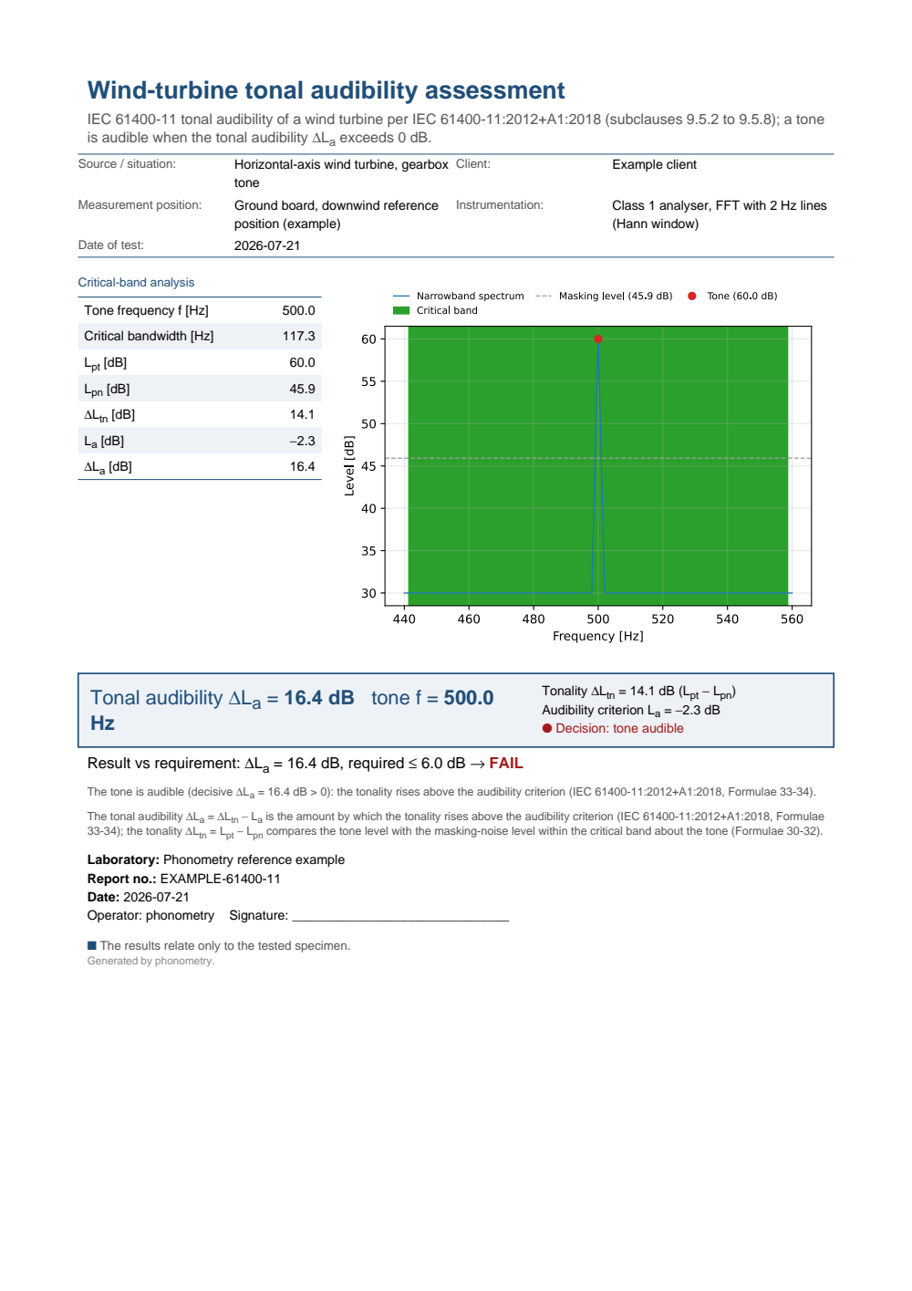
One-page wind-turbine tonal-audibility fiche: a metadata header, a critical-band analysis table (tone frequency 500.0 Hz, critical bandwidth 117.3 Hz, tone level Lpt = 60.0 dB, masking-noise level Lpn = 45.9 dB, tonality ΔL_tn = 14.1 dB, audibility criterion La = -2.3 dB) beside the narrowband-spectrum plot with the critical band shaded and the masking level drawn, the boxed tonal audibility ΔL_a = 16.4 dB at the 500.0 Hz tone with the decision that the tone is audible, and a FAIL verdict against a maximum acceptable audibility of 6.0 dB.
What this guide covers
Section titled “What this guide covers”Covered
The closed-form quantities of IEC 61400-11:2012+A1:2018:
slant_distance(Formulae 1 and 2),apparent_sound_power_level(Formula 26) and the tonal-audibility chain of subclauses 9.5.2 to 9.5.8 throughwind_turbine_tonality, with its.report()fiche. The instrumentation and position requirements of clauses 6 and 7 are documented above as the conditions those formulae assume, and the measurement-position tolerances are drawn.Not covered
The measurement campaign itself: the 10 s averaging, the 0,5 m/s wind-speed binning with its 10 + 10 periods, the background correction, the interpolation to bin centres, the Formula (29) mapping to m and the uncertainty budget of clause 9.3 all operate on whole campaigns and are the user’s. The declaration route of IEC TS 61400-14, which turns a batch of measured machines into the single number a planning authority receives, is not implemented either. And two things a wind-turbine reader often arrives looking for are outside IEC 61400-11 altogether: amplitude modulation (the “swish”, which is folded into and rated nowhere in this standard) and infrasound. Both are listed in 7.2.1 as optional measurements with no rating method attached, so their assessment falls to national guidance; the psychoacoustic route to them starts at Fluctuation strength and roughness and at Special weightings for the G-weighted infrasound level.
References
Section titled “References”- International Electrotechnical Commission. (2005). Wind turbines — Part 14: Declaration of apparent sound power level and tonality values (IEC TS 61400-14:2005). How a manufacturer turns IEC 61400-11 measurements of a batch of turbines into declared values with a stated uncertainty, the number a planning authority actually receives.
- International Electrotechnical Commission. (2018). Wind turbines — Part 11: Acoustic noise measurement techniques (IEC 61400-11:2012+AMD1:2018 CSV). The implemented edition: the measurement geometry, the wind-speed binning and the tonal-audibility chain (apparent sound power Formula 26, critical bandwidth Formula 30, masking level Formula 31, tonality/audibility Formulae 32-34). The full measurement pipeline is out of scope here.
- International Organization for Standardization. (2017). Acoustics — Description, measurement and assessment of environmental noise — Part 2: Determination of sound pressure levels (ISO 1996-2:2017). The tonal-audibility criterion the IEC method reuses comes from the Annex C of its 2007 edition (the 2017 edition carries the tonal methods in Annexes J and K), and its Table J.1 mapping, tonal_adjustment_from_mean_audibility, is the one that consumes the bin-mean audibility.