Sound Quality Metrics

Two sounds of equal loudness can still differ in how sharp, how tonal, how rough or how strongly fluctuating they are. This page covers the sound-quality metrics that complement loudness: sharpness (DIN 45692) and the ECMA-418-2 tonality, roughness and fluctuation strength of the Sottek Hearing Model. Loudness itself lives in Loudness; the ECMA-418-2 loudness that shares the same auditory front-end lives in Advanced Loudness.

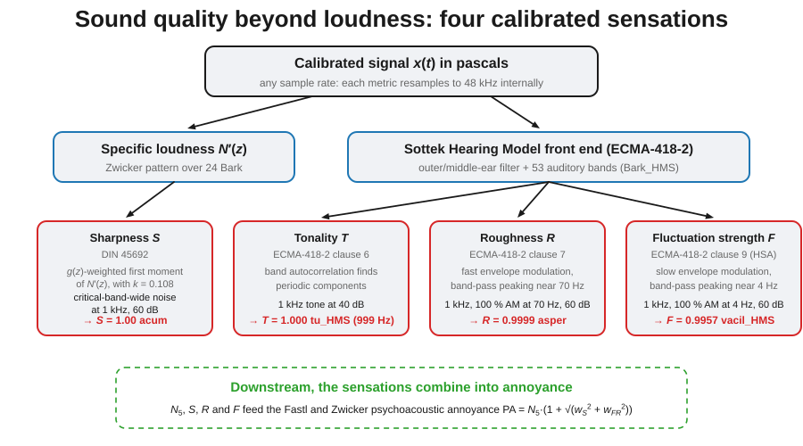
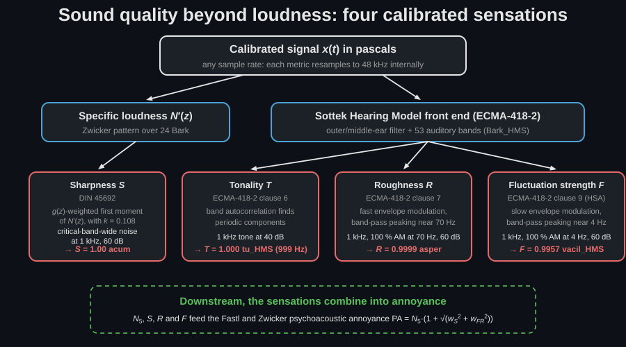
The four metrics form one family: a single calibrated signal splits across two auditory front ends, and every branch is anchored to a reference sound whose normative target is exactly 1. The diagram maps the family with the values the library actually computes for each reference (rounded results such as 0.9999 asper and 0.9957 vacil_HMS sit against that target of 1).

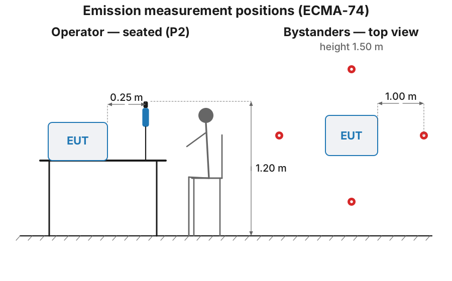
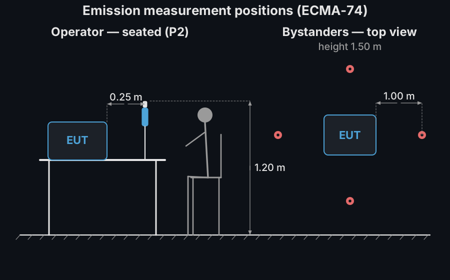
Recording the signal these metrics need

ECMA-418-2 is a calculation applied to a recording, and clause 2 makes the recording part of conformance: measurements conform only if they are taken in conformity with ECMA-74 and carried out at 48 kHz, or resampled to it. That pulls in a test environment qualified to ISO 11201 accuracy grade 2, a declared operating mode, and the microphone at the ECMA-74 positions — the operator position 0.25 m from the reference box at 1.20 m seated or 1.50 m standing, or at least four bystander positions 1.00 m out and 1.50 m up — with the background noise measured with the equipment off and a calibrator applied before and after. The positions are the same ones the tone-prominence guide works from, and it states them in full:

How long the record has to be is the question the three ECMA metrics answer differently, and no snippet on this page would tell you: the measurement interval must cover at least three operational cycles, or the complete sequence for equipment that varies, and on top of that each metric has a settling time of its own. Tonality settles within about a second for a steady tone, because the autocorrelation works inside each block. Roughness needs a couple of seconds: its single value is the 90th percentile of $R(l_{50})$ over the blocks that survive the initial transient, and the trace drawn further down takes about 0.5 s to reach its plateau. Fluctuation strength needs the longest record, of the order of ten seconds, because it resolves modulation rates near 4 Hz — its trace is still climbing at 3 s and only settles around 4 s, so a two-second excerpt contains a handful of modulation periods and reads low.

Draw the consequence: values computed on short clips are biased low for $R$ and $F$, so compare only values computed over comparable durations, and state the analysis length beside the value as a matter of course. The snippets below use 1.2 s, 2.0 s and 8.0 s for exactly this reason.

Caution

A binaural or artificial-head recording must already be free-field or diffuse-field equalized before it reaches tonality_ecma, roughness_ecma or fluctuation_strength_ecma. Clause 5.1.3 assumes it: in an ideal field the two equalized channels correspond to a microphone at the centre of the now absent artificial head, which is what the field= filter is built for. Feeding an unequalized manikin recording applies the outer-ear filter twice. Each channel is analysed separately, since the binaural combinations are not implemented.

Sharpness in acum (DIN 45692)

Two sounds can be equally loud yet one feels “sharper” (hissy, metallic) because its loudness sits higher on the Bark scale. Sharpness is the $g(z)$-weighted first moment of the specific loudness pattern:

$$S=k\frac{{\int }_0^{24}{N}^{\prime }(z)g(z)zdz}{{\int }_0^{24}{N}^{\prime }(z)dz}\text{acum}$$

with $g(z)=1$ up to 15.8 Bark and rising exponentially beyond, and $k$ normalized so the reference sound (critical-band-wide noise at 1 kHz, 60 dB) is exactly 1.00 acum (DIN 45692 clause 6; the derived $k=0.108$ sits inside the normative window 0.105–0.115).

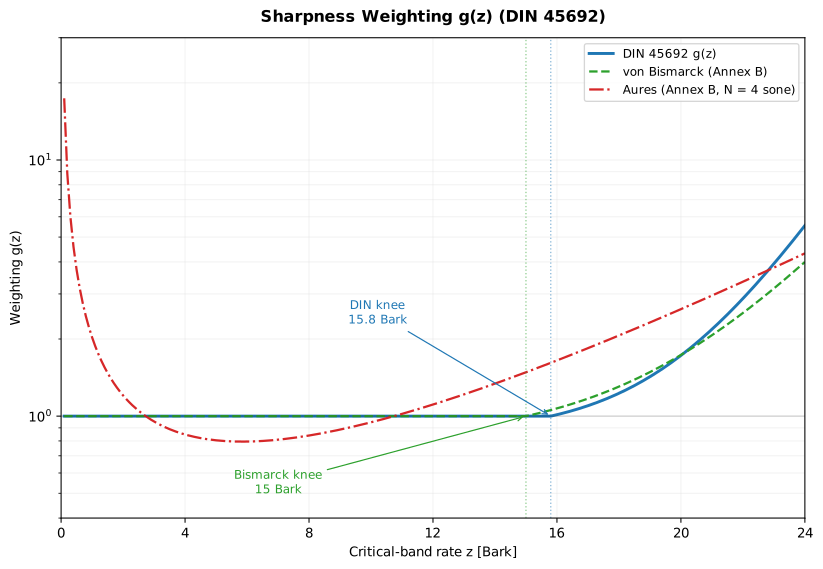
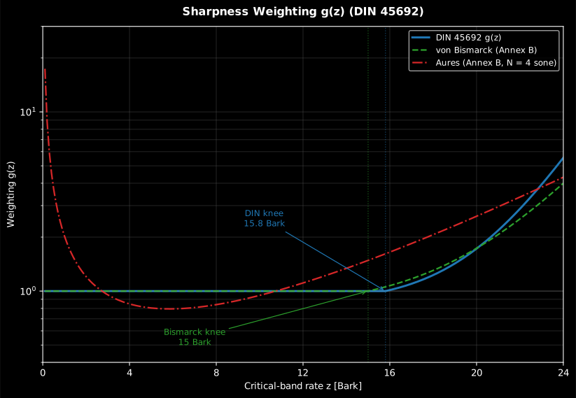
The three weightings. All are flat to about 15 Bark and rise exponentially above it, which is what makes high-frequency loudness count for more; the Aures curve, unlike the other two, moves with the total loudness.

Show the code for this figure

import matplotlib.pyplot as plt
import numpy as np

# DIN 45692 sharpness weighting g(z): Eq. (1) plus the informative Annex B variants
z = np.arange(1, 241) * 0.1                     # Bark bins, 0.1 .. 24.0
g_din = np.where(z > 15.8, 0.15 * np.exp(0.42 * (z - 15.8)) + 0.85, 1.0)
g_bis = np.where(z > 15.0, 0.2 * np.exp(0.308 * (z - 15.0)) + 0.8, 1.0)
n = 4.0                                         # Aures depends on the total loudness (sone)
g_aures = 0.078 * np.exp(0.171 * z) / z * (n / np.log(n * 0.05 + 1.0))

fig, ax = plt.subplots()
ax.semilogy(z, g_din, label="DIN 45692 g(z)")
ax.semilogy(z, g_bis, "--", label="von Bismarck (Annex B)")
ax.semilogy(z, g_aures, "-.", label="Aures (Annex B, N = 4 sone)")
ax.axvline(15.8, linestyle=":", color="0.5")    # DIN knee: g rises beyond 15.8 Bark
ax.set(xlabel="Critical-band rate z [Bark]", ylabel="Weighting g(z)")
ax.grid(True, which="both", alpha=0.3)
ax.legend()
plt.show()

import numpy as np
from phonometry import psychoacoustics

# A raw recording plus its calibration so the guide runs standalone
fs = 48000
x = 0.2 * np.sin(2 * np.pi * 1000 * np.arange(fs) / fs)   # any recording (digital units)
sens = 1.0                                                # calibration_factor to pascals

s = psychoacoustics.sharpness_din(x, fs, calibration_factor=sens)      # acum
s_aures = psychoacoustics.sharpness_din(x, fs, method="aures")        # Annex B variant
print(f"S = {s:.2f} acum  (Aures {s_aures:.2f} acum)")                # 1.03 acum (Aures 1.23)

CI verifies the Table A.2 target values (0.38 acum at 250 Hz up to 2.82 acum at 4 kHz) within the standard’s 5 % / 0.05 acum tolerance.

Sharpness is a position, not a level. Both the numerator and the denominator of $S$ contain $N^{\prime }(z)$, so the level cancels: what the ratio answers is where on the Bark axis this sound’s loudness sits. That is why DIN 45692 clause 6 fixes the reference sound and every one of its verification signals at the same loudness — 4 sone — and why comparing the sharpness of two sounds of very different loudness is close to meaningless. The range is worth memorising: a critical band of noise at 250 Hz reads about 0.4 acum, the 1 kHz reference exactly 1 acum, a critical band at 4 kHz about 2.8 acum, and broadband product noise usually lands between 1 and 3 acum, with the hiss-dominated sounds customers call shrill above 2 acum.

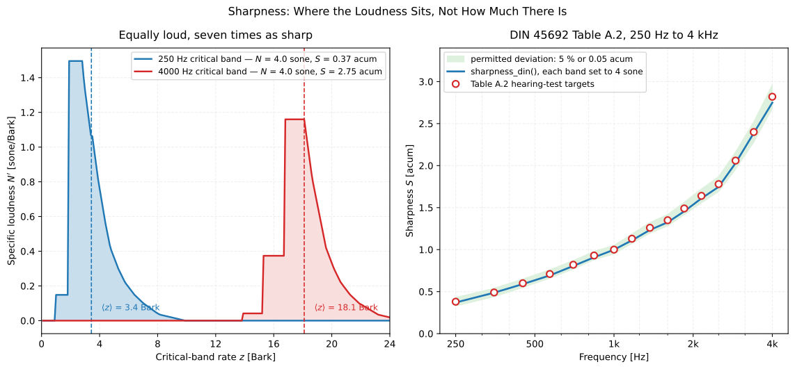
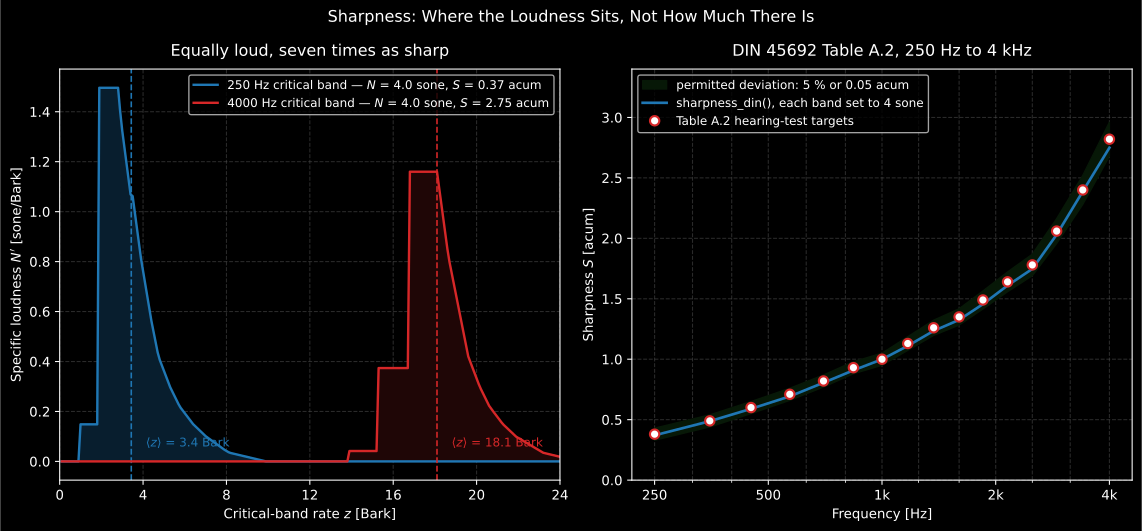
Equal loudness, seven times the sharpness. Both patterns integrate to 4 sone; what differs is where they sit, and that is the whole content of the metric. Right: the same computation against the standard’s own hearing-test targets, every point inside the permitted deviation.

Show the code for this figure

import numpy as np
from scipy import signal as sp_signal

# `psychoacoustics` is imported by the snippets above.
# One DIN 45692 Table A.1 critical band of noise, at a chosen band level.
def critical_band_noise(f_low, f_high, level_db):
    rng = np.random.default_rng(7)
    sos = sp_signal.butter(8, [f_low, f_high], btype="band", fs=48000, output="sos")
    band = sp_signal.sosfilt(sos, rng.standard_normal(48000 * 2))
    band /= np.sqrt(np.mean(band**2))
    return band * 2e-5 * 10 ** (level_db / 20)

# Table A.2 compares signals of equal loudness, so set each band to 4 sone.
def level_for_four_sone(f_low, f_high):
    low, high = 30.0, 95.0
    for _ in range(14):
        mid = (low + high) / 2
        loud = psychoacoustics.loudness_zwicker(
            critical_band_noise(f_low, f_high, mid), 48000, stationary=True).loudness
        low, high = (mid, high) if loud < 4.0 else (low, mid)
    return (low + high) / 2

for centre, f_low, f_high, target in [(250.0, 200.0, 300.0, 0.38),
                                      (4000.0, 3700.0, 4400.0, 2.82)]:
    band = critical_band_noise(f_low, f_high, level_for_four_sone(f_low, f_high))
    print(centre, round(float(psychoacoustics.sharpness_din(band, 48000)), 2), target)
#   250.0 0.37 0.38
#   4000.0 2.75 2.82

Which variant. The DIN weighting is loudness-independent, a good approximation near the 4 sone it was calibrated at but under-reading the sharpness listeners report for very quiet sounds; the informative Aures weighting scales with the total loudness and is therefore the variant to reach for when the sounds being compared differ markedly in loudness. Von Bismarck is the historical curve with its knee at 15 Bark, kept for continuity with older data. For a sound whose spectrum moves, DIN 45692 clause 6 recommends quoting the percentile $S_{50}$ over the analysis rather than one instantaneous value.

sharpness_din() parameters

Parameter	Type	Units	Range / default	Notes
x	1D array	Pa (after calibration)	non-empty	The signal the specific-loudness pattern is computed from
fs	int	Hz	> 0
field	str	—	'free' (default) / 'diffuse'	The ISO 532-1 sound-field correction, inherited from the loudness stage
method	str	—	'din' (default, clause 6) / 'bismarck' / 'aures'	The $g(z)$ weighting; the last two are Annex B
calibration_factor	float	Pa per digital unit	default 1.0	From sensitivity()

Unlike the three ECMA metrics below, sharpness_din() returns a plain float in acum, not a result object with its own .plot().

Tonality (ECMA-418-2)

A tonal component (a whistle, a fan’s blade-passing tone) stands out even at low level. ECMA-418-2 quantifies it from the autocorrelation function (ACF) of each band’s rectified signal: a periodic (tonal) component keeps a high ACF at nonzero lag, and the tonal-to-noise loudness ratio drives the specific tonality $T^{\prime }(z)$. The single value $T$ is in tu_HMS, calibrated so a 1 kHz/40 dB tone is $\approx 1$ tu_HMS; the result also tracks the tonal frequency $f_{\text{ton}}$ per band.

import numpy as np
from phonometry import psychoacoustics

fs = 48000
t = np.arange(int(1.2 * fs)) / fs
x = np.sqrt(2) * 2e-5 * 10 ** (40 / 20) * np.sin(2 * np.pi * 1000 * t)

res = psychoacoustics.tonality_ecma(x, fs, field="free")
peak = int(np.argmax(res.specific_tonality))
print(f"T = {res.tonality:.3f} tu_HMS")                    # 1.000 tu_HMS
print(f"f_ton = {res.tonal_frequencies[peak]:.0f} Hz")     # 999 Hz

res.plot()   # average specific tonality T'(z) + time-dependent T(l)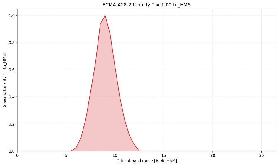

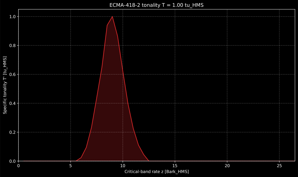
The calibration anchor seen band by band: a 1 kHz tone at 40 dB puts all of its tonality in one critical band, which is what makes the tonal-to-noise loudness ratio large there and negligible everywhere else.

Show the code for this figure

import matplotlib.pyplot as plt
import numpy as np
from phonometry import psychoacoustics

# The calibration anchor: a 1 kHz tone at 40 dB SPL is about 1 tu_HMS.
fs = 48000
t = np.arange(int(1.2 * fs)) / fs
x = np.sqrt(2) * 2e-5 * 10 ** (40 / 20) * np.sin(2 * np.pi * 1000 * t)
res = psychoacoustics.tonality_ecma(x, fs, field="free")

# One line: passing an axes draws the specific-tonality panel alone.
fig, ax = plt.subplots()
res.plot(ax=ax)
plt.show()

# Or draw T'(z) by hand against the critical-band-rate scale:
fig, ax = plt.subplots()
ax.fill_between(res.bark, res.specific_tonality, alpha=0.3, color="#d62728")
ax.plot(res.bark, res.specific_tonality, color="#d62728")
ax.set_xlabel("Critical-band rate z [Bark_HMS]")
ax.set_ylabel("Specific tonality T' [tu_HMS]")
plt.show()

The concentration is what distinguishes a tonal sound from a broadband one of the same loudness: the autocorrelation stage finds a periodic component in one band and almost nothing in the others. A fan with a blade-passing tone and a harmonic series shows several such peaks; a hiss shows a flat, low pattern. Calling .plot() without an axes adds the time-dependent $T(l)$ panel, which is where an intermittent tone shows up.

Reading a tonality. ECMA-418-2 clause 6.3 attaches its prominence criterion to the pattern, not to the single value: a tonal component in band $z_{\text{tonal}}$ counts as prominent when the specific tonality $T^{\prime }(z_{\text{tonal}})$ exceeds 0.4 tu_HMS, is a local maximum along $z$, and carries a tonal frequency lying between its neighbouring band centres. So a prominence statement is read from specific_tonality and tonal_frequencies, never from $T$ alone. The standard attaches no limit to the overall $T$, which makes it a magnitude for comparing designs rather than a pass/fail test; the test is the ECMA-418-1 tone-to-noise and prominence ratio of Prominent Discrete Tones.

tonality_ecma() parameters

Parameter	Type	Units	Range / default	Notes
signal_in	1D array	Pa	non-empty	Calibrated pressure signal
fs	float	Hz	> 0	Resampled to 48 kHz internally if needed
field	str	—	'free' (default) / 'diffuse'	Outer/middle-ear filter
f_low	float, optional	Hz	default None	Lower edge of a user band for the $T(l)$ search
f_high	float, optional	Hz	default None	Upper edge of the user band

Returns an EcmaTonality: tonality ($T$, tu_HMS), specific_tonality ($T^{\prime }(z)$, 53 bands), bark, centre_frequencies, tonal_frequencies ($f_{\text{ton},z}$), time, tonality_vs_time ($T(l)$), tonal_frequency_vs_time, field.

Roughness in asper (ECMA-418-2)

Roughness is the harsh, buzzing sensation of fast amplitude modulation (roughly 20–300 Hz, peaking near 70 Hz): the quality of a diesel idle or a distorted loudspeaker. ECMA-418-2 extracts each band’s envelope, weights its modulation spectrum by modulation rate and depth, and correlates the modulation across bands; the result $R$ is in asper. The reference sound (1 kHz carrier, 100 % amplitude-modulated at 70 Hz, overall level 60 dB SPL) is defined as 1 asper; this clean-room implementation returns 0.9999 asper with the tabulated calibration constant $c_R$ (Formula 104) used without reverse-fitting to the target.

import numpy as np
from phonometry import psychoacoustics

fs = 48000
t = np.arange(int(2.0 * fs)) / fs
x = (1.0 + np.cos(2 * np.pi * 70 * t)) * np.sin(2 * np.pi * 1000 * t)
x *= 2e-5 * 10 ** (60 / 20) / np.sqrt(np.mean(x**2))   # overall 60 dB SPL

res = psychoacoustics.roughness_ecma(x, fs, field="free")
print(f"R = {res.roughness:.4f} asper")   # 0.9999 asper (reference: 1 asper)

res.plot()   # time-dependent roughness R(l50) + specific-roughness heatmap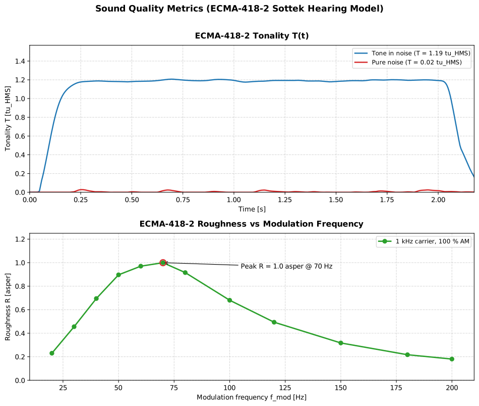

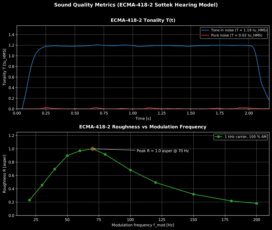
The two sensations, each read the way its clause defines it: tonality as a time trace, which separates a tone in noise from the noise alone, and roughness as a function of modulation rate, whose 70 Hz peak on a fully modulated 1 kHz carrier at 60 dB is the calibration point of the asper.

Show the code for this figure

import matplotlib.pyplot as plt
import numpy as np
from phonometry import psychoacoustics

fs, p0 = 48000, 2e-5

# Top panel: tonality T(t) of a 1 kHz tone in noise against the noise alone,
# each component at 50 dB SPL over 2 s.
t = np.arange(int(2.0 * fs)) / fs
rng = np.random.default_rng(2026)
noise = rng.standard_normal(t.size)
noise *= p0 * 10 ** (50 / 20) / np.sqrt(np.mean(noise**2))
tone = p0 * 10 ** (50 / 20) * np.sqrt(2) * np.sin(2 * np.pi * 1000 * t)
tin = psychoacoustics.tonality_ecma(tone + noise, fs)
pn = psychoacoustics.tonality_ecma(noise, fs)

# Bottom panel: roughness of a 1 kHz carrier at 100 % AM, swept over the
# modulation frequency (1 s per point at 60 dB SPL).
tm = np.arange(fs) / fs
fmods = np.array([20.0, 30, 40, 50, 60, 70, 80, 100, 120, 150, 180, 200])
r = []
for fm in fmods:
    am = (1 + np.sin(2 * np.pi * fm * tm)) * np.sin(2 * np.pi * 1000 * tm)
    am *= p0 * 10 ** (60 / 20) / np.sqrt(np.mean(am**2))
    r.append(psychoacoustics.roughness_ecma(am, fs).roughness)

fig, (ax0, ax1) = plt.subplots(2, 1, figsize=(10, 8.5))
ax0.plot(tin.time, tin.tonality_vs_time,
         label=f"Tone in noise (T = {tin.tonality:.2f} tu_HMS)")   # 1.19
ax0.plot(pn.time, pn.tonality_vs_time,
         label=f"Pure noise (T = {pn.tonality:.2f} tu_HMS)")       # 0.02
ax0.set(xlabel="Time [s]", ylabel="Tonality T [tu_HMS]")
ax0.legend()
ax1.plot(fmods, r, "o-", label="1 kHz carrier, 100 % AM")          # peak 1.0 asper
ax1.set(xlabel="Modulation frequency f_mod [Hz]", ylabel="Roughness R [asper]")
ax1.legend()
plt.show()

Reading a roughness. Clause 7.2 gives the criterion the tonality section withholds: a signal has prominent roughness when the single value $R$ — the 90th percentile of the time-dependent $R(l_{50})$, not its mean — exceeds 0.2 asper. The percentile matters: short bursts of harshness are not averaged away, which also means the record has to be long enough for that percentile to settle. The figure below is the reference sound seen the two ways the result object carries it.

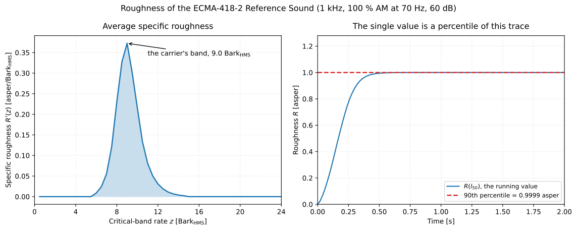
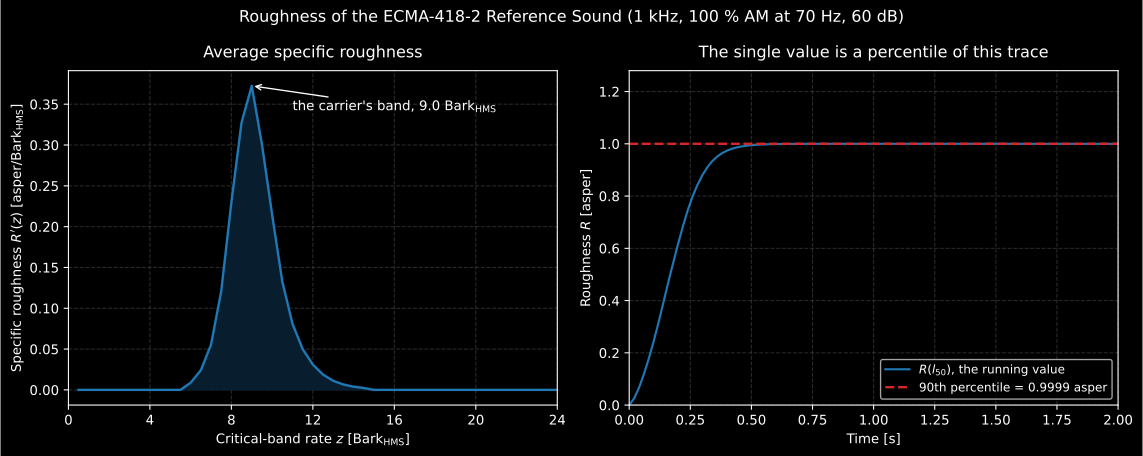
The reference sound, band by band and instant by instant. The single value is the dashed line: a percentile of the trace on the right, integrated from the pattern on the left. The half-second run-up is why a two-second record is the practical minimum.

Show the code for this figure

import matplotlib.pyplot as plt

# `res` is the roughness result of the snippet above.
fig, (ax0, ax1) = plt.subplots(1, 2, figsize=(12, 4.8))
ax0.plot(res.bark, res.specific_roughness)
ax0.set(xlabel="Critical-band rate z [Bark_HMS]",
        ylabel="Specific roughness R'(z) [asper/Bark_HMS]")
ax1.plot(res.time, res.roughness_vs_time)
ax1.axhline(res.roughness, linestyle="--")     # the 90th percentile
ax1.set(xlabel="Time [s]", ylabel="Roughness R [asper]")
plt.show()

roughness_ecma() parameters

Parameter	Type	Units	Range / default	Notes
signal_in	1D array	Pa	non-empty	Calibrated pressure signal
fs	float	Hz	> 0	Resampled to 48 kHz internally if needed
field	str	—	'free' (default) / 'diffuse'	Outer/middle-ear filter

Returns an EcmaRoughness: roughness ($R$, asper, the 90th percentile of $R(l_{50})$), specific_roughness ($R^{\prime }(z)$, 53 bands), bark, centre_frequencies, time, roughness_vs_time ($R(l_{50})$), specific_roughness_vs_time ((n_times, 53) array), field.

Fluctuation strength in vacil_HMS (ECMA-418-2)

Fluctuation strength is the slow, wobbling sensation of amplitude or frequency modulation below about 20 Hz: a siren, beating tones, speech at syllable rate. It is the slow counterpart of roughness: the same hearing model splits envelope modulation into a slow band-pass peaking near 4 Hz (fluctuation strength, in vacil_HMS) and a fast one peaking near 70 Hz (roughness). ECMA-418-2 Clause 9 analyses each band’s envelope with High-resolution Spectral Analysis (HSA), a least-squares fit of window-kernel spectral line pairs that resolves modulation rates far below the DFT bin width, using envelope-dependent analysis windows that skip quieter periods, then weights the dominant harmonic complex and scales it with an HSA-based specific loudness. The reference sound (1 kHz carrier, 100 % amplitude-modulated at 4 Hz, overall level 60 dB SPL) is defined as 1 vacil_HMS; this clean-room implementation converges to 0.9958 vacil_HMS by 12 s with the tabulated calibration constant $c_F$ (Formula 163) used without reverse-fitting to the target (the 8 s example below prints 0.9957). A signal whose single value $F$ exceeds 0.2 vacil_HMS has a prominent fluctuation strength (Clause 9.2).

import numpy as np
from phonometry import psychoacoustics

fs = 48000
t = np.arange(int(8.0 * fs)) / fs
x = (1.0 + np.cos(2 * np.pi * 4 * t)) * np.sin(2 * np.pi * 1000 * t)
x *= 2e-5 * 10 ** (60 / 20) / np.sqrt(np.mean(x**2))   # overall 60 dB SPL

res = psychoacoustics.fluctuation_strength_ecma(x, fs, field="free")
print(f"F = {res.fluctuation_strength:.4f} vacil_HMS")   # 0.9957 vacil_HMS (reference: 1 vacil_HMS)

res.plot()   # time-dependent F(l50) + specific-fluctuation-strength heatmap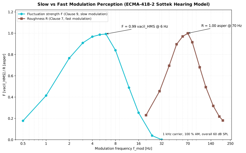

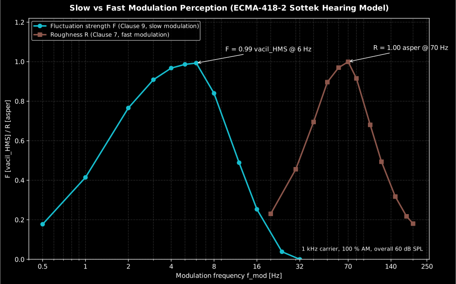
Two band-passes on the same envelope. The same modulated carrier is heard as fluctuation below about 20 Hz and as roughness above it, which is why the two metrics divide the modulation axis between them rather than competing on it.

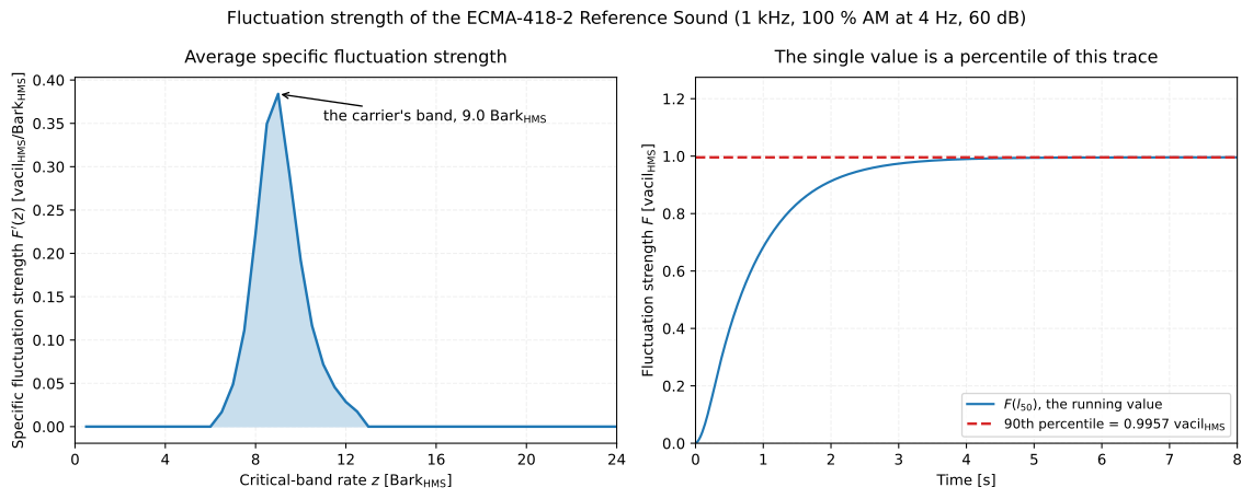
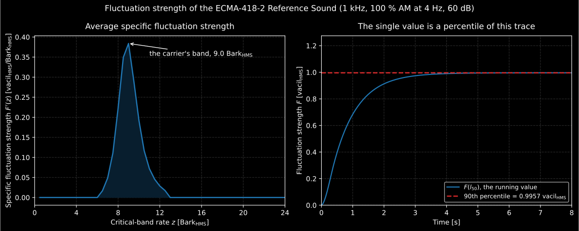
The same two views for the slow sensation, and the reason this metric needs the longest record on the page: the trace is still climbing at 3 s. A two-second excerpt of this very reference sound would read well below 1 vacil_HMS.

Show the code for this figure

import matplotlib.pyplot as plt
import numpy as np
from phonometry import psychoacoustics

fs = 48000
t = np.arange(int(3.0 * fs)) / fs
carrier = np.sin(2 * np.pi * 1000 * t)

def am_tone(fmod):
    # 100 % AM at an overall level of 60 dB SPL (the Clause 7/9 convention)
    x = (1.0 + np.sin(2 * np.pi * fmod * t)) * carrier
    return x * 2e-5 * 10 ** (60 / 20) / np.sqrt(np.mean(x**2))

fm_slow = [0.5, 1, 2, 4, 8, 16, 32]
fm_fast = [20, 40, 70, 100, 150, 200]
f_vals = [psychoacoustics.fluctuation_strength_ecma(am_tone(fm), fs).fluctuation_strength
          for fm in fm_slow]
r_vals = [psychoacoustics.roughness_ecma(am_tone(fm), fs).roughness for fm in fm_fast]

fig, ax = plt.subplots()
ax.semilogx(fm_slow, f_vals, "o-", label="Fluctuation strength F [vacil_HMS]")
ax.semilogx(fm_fast, r_vals, "s-", label="Roughness R [asper]")
ax.set(xlabel="Modulation frequency [Hz]", ylabel="F [vacil_HMS] / R [asper]")
ax.legend()
plt.show()

fluctuation_strength_ecma() parameters

Parameter	Type	Units	Range / default	Notes
signal_in	1D array	Pa	non-empty	Calibrated pressure signal
fs	float	Hz	> 0	Resampled to 48 kHz internally if needed
field	str	—	'free' (default) / 'diffuse'	Outer/middle-ear filter

Returns an EcmaFluctuationStrength: fluctuation_strength ($F$, vacil_HMS, the 90th percentile of $F(l_{50})$), specific_fluctuation_strength ($F^{\prime }(z)$, 53 bands), bark, centre_frequencies, time, fluctuation_strength_vs_time ($F(l_{50})$), specific_fluctuation_strength_vs_time ((n_times, 53) array), field.

The Fastl & Zwicker fluctuation-strength models (closed form for AM broadband noise and the Osses 2016 signal model) live in Psychoacoustic Annoyance; this Clause 9 metric is the normative Sottek-model counterpart.

See Prominent Discrete Tones for the ECMA-418-1 TNR/PR prominence verdicts, Speech Transmission Index for STI/STIPA, and Theory for the underlying math.

What this guide covers

• Covered

  DIN 45692:2009 through sharpness_din(): the clause 6 weighting over the ISO 532-1 specific-loudness pattern, plus the informative Annex B von Bismarck and Aures variants, with the Table A.2 targets checked in CI. ECMA-418-2:2025 on the shared clause 5 auditory front-end: the clause 6.2 tonality output stages (tonality_ecma()), the clause 7 roughness chain (roughness_ecma()) and the clause 9 HSA fluctuation strength (fluctuation_strength_ecma()). Each uses the standard’s tabulated calibration constant, not a reverse fit to the reference sound.

• Not covered

  The three ECMA-418-2 entry points are monaural: the binaural quadratic-mean combinations of Formula 112 (clause 7.1.11) and Formula 170 (clause 9.1.15) are not implemented, so analyse each channel separately. The optional entropy weighting of clause 7.1.6 needs an external rotational-speed signal and is left out, as is the ±0.25 % adjustment of $c_F$ that footnote 47 permits. The ECMA-418-2 loudness that shares this front-end lives in Advanced Loudness, and the Fastl and Zwicker fluctuation-strength models in Psychoacoustic Annoyance.

See also

• API reference: psychoacoustics.quality.sharpness, psychoacoustics.quality.tonality_ecma, psychoacoustics.quality.roughness_ecma and psychoacoustics.quality.fluctuation_strength_ecma.
• Theory: Advanced loudness models and sound quality: the specific-loudness pattern the sharpness, roughness and fluctuation-strength metrics are all built on.

References

• Deutsches Institut für Normung. (2009). Messtechnische Simulation der Hörempfindung Schärfe (DIN 45692:2009). Sharpness in acum: the clause 6 weighting, the Annex B von Bismarck and Aures variants and the Table A.2 targets.
• Ecma International. (2025). Psychoacoustic metrics for ITT equipment — Part 2 (methods for describing human perception based on the Sottek Hearing Model) (ECMA-418-2:2025). The Sottek Hearing Model tonality (tu_HMS, clause 6), roughness (asper, clause 7) and fluctuation strength (vacil_HMS, clause 9, the HSA-based envelope analysis).
• Fastl, H., & Zwicker, E. (2007). Psychoacoustics: Facts and models (3rd ed.). Springer. https://doi.org/10.1007/978-3-540-68888-4The psychoacoustics of the sensations quantified on this page: the high-frequency emphasis behind sharpness and the fast-modulation percept behind roughness.