Loudness

Level metrics tell you how much sound pressure there is; loudness tells you how loud a listener actually perceives it. This page covers the reference method, loudness in sones by Zwicker (ISO 532-1), plus the equal-loudness contours of pure tones (ISO 226); the newer model families, Moore-Glasberg (ISO 532-2/-3) and the Sottek Hearing Model loudness (ECMA-418-2), are Advanced Loudness. Sharpness, tonality and roughness live in Sound Quality Metrics; speech metrics in Speech Transmission Index and Speech Intelligibility Index.

How do I compute ISO 532-1 Zwicker loudness in Python?

Call psychoacoustics.loudness_zwicker(x, fs, calibration_factor=sens) on a calibrated recording. If you only have a spectrum, use loudness_zwicker_from_spectrum(levels_28) with the 28 one-third-octave band levels from 25 Hz to 12.5 kHz. Either result carries loudness_level in phons and loudness in sones — the single stationary $N$ with stationary=True, the peak $N_{\text{max}}$ of the loudness trace otherwise — plus the reporting percentiles n5 and n10 for a time-varying run.

Loudness in sones (ISO 532-1, Zwicker)

Decibels compress perception: 10 dB more reads as twice as loud, and two sounds with the same dB(A) can differ audibly depending on how their energy spreads over the ear’s critical bands. The Zwicker method models the hearing chain explicitly (outer/middle-ear transmission, critical-band analysis on the 24 Bark scale, level-dependent masking slopes) and outputs loudness $N$ in sones, a ratio scale: 4 sones is twice as loud as 2 sones. By definition a 1 kHz tone at 40 dB SPL is 1 sone, and every +10 phon doubles the sone value.

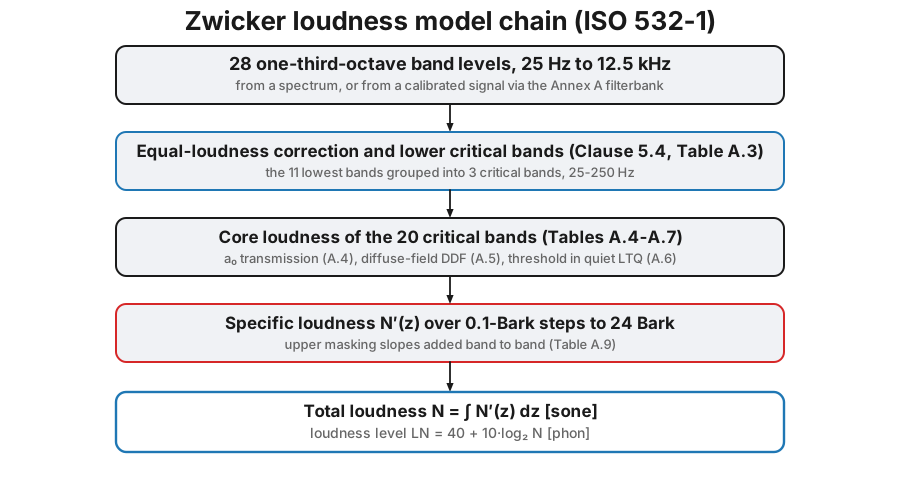
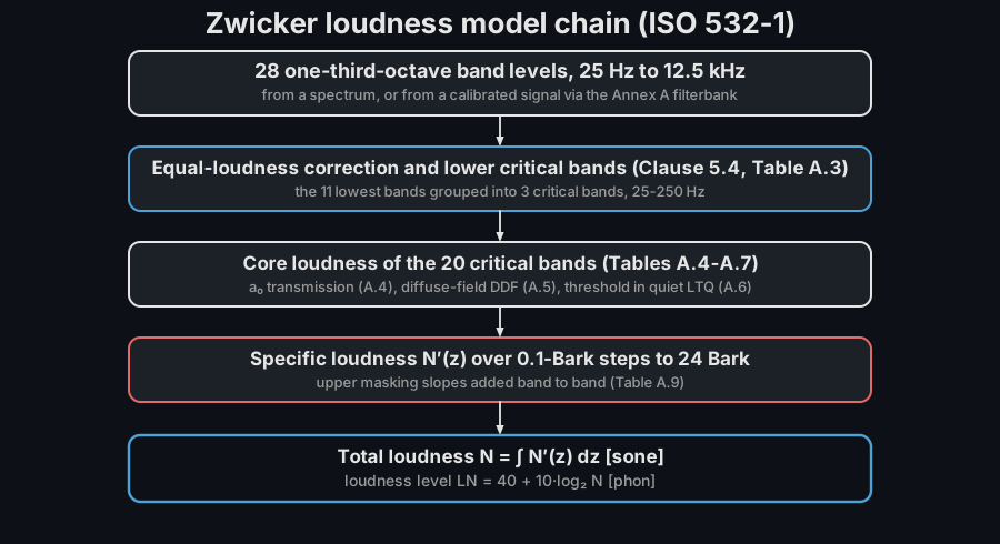
The animation below shows that integration at work: as the band level of a 1 kHz narrowband sound steps up, the specific-loudness pattern $N^{\prime }(z)$ grows along the Bark axis and the area under it is the total loudness in sones.

The specific-loudness pattern of a 1 kHz narrowband sound builds along the Bark axis as the band level steps from 45 to 85 dB, and the area under the pattern integrates to the total loudness in sones.

Download the animation (WebM)

The specific-loudness pattern of a 1 kHz narrowband sound builds along the Bark axis as the band level steps from 45 to 85 dB, and the area under the pattern integrates to the total loudness in sones.

Download the animation (WebM)

Measuring the input (clause 4)

Loudness is an absolute-level quantity: nothing in it cancels, so an uncalibrated or A-weighted recording produces a plausible number that is simply wrong, and the result carries no sign of it. ISO 532-1 therefore specifies the input before it specifies the model.

The chain. A microphone, preamplifier and amplifier meeting IEC 61672-1:2013 class 1, and a field calibration that turns digital units into pascals — that factor is what calibration_factor expects, and Calibration is where it comes from. Clause 4 fixes the sampling rate of the reference implementation at 48 kHz; other rates are resampled to it, which the library does internally. For the band-level entry point, the 28 one-third-octave levels must come from filters conforming to IEC 61260-1:2014 class 1 with centre frequencies from 25 Hz to 12.5 kHz.

Two rules about the samples themselves. No frequency weighting of any kind: definition 3.2 Note 1 states that weightings such as A-weighting shall not be used for loudness calculation, because the model applies the ear’s own weighting internally and an A-weighted input weights it twice. And true sound pressure, not normalised or peak-scaled data (clause 4, “correct sound pressure values, no normalized data”). The sens = 1.0 in the snippets below is a placeholder that keeps this page runnable, not a default worth keeping: get the calibration wrong by 10 dB and the reported loudness doubles or halves (13.1 sone becomes 26.6 or 6.5 on the example signal), which dwarfs every difference between the models on the next page.

Where the microphone goes. Definition 3.19 Note 2 puts it at the point where the centre of the listener’s head would be, with the listener absent; that is what makes the calculated loudness the loudness of a diotic presentation, the same sound at both ears. The geometry drawn below is the ECMA-74 bystander position — 1.00 m from the reference box, 1.50 m above the reflecting plane — because ISO 532-1 prescribes no distance of its own and takes it from whichever emission standard applies.

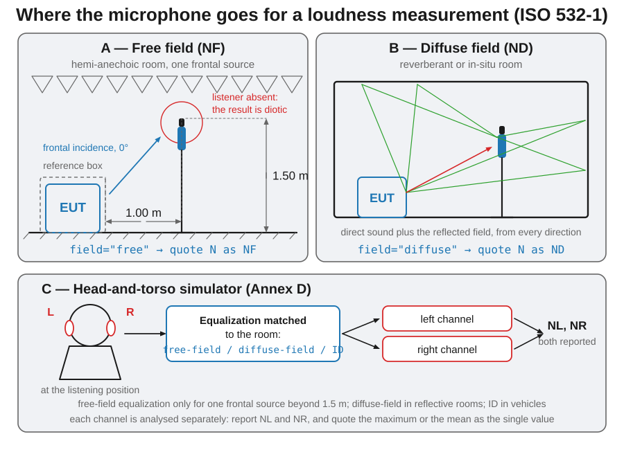
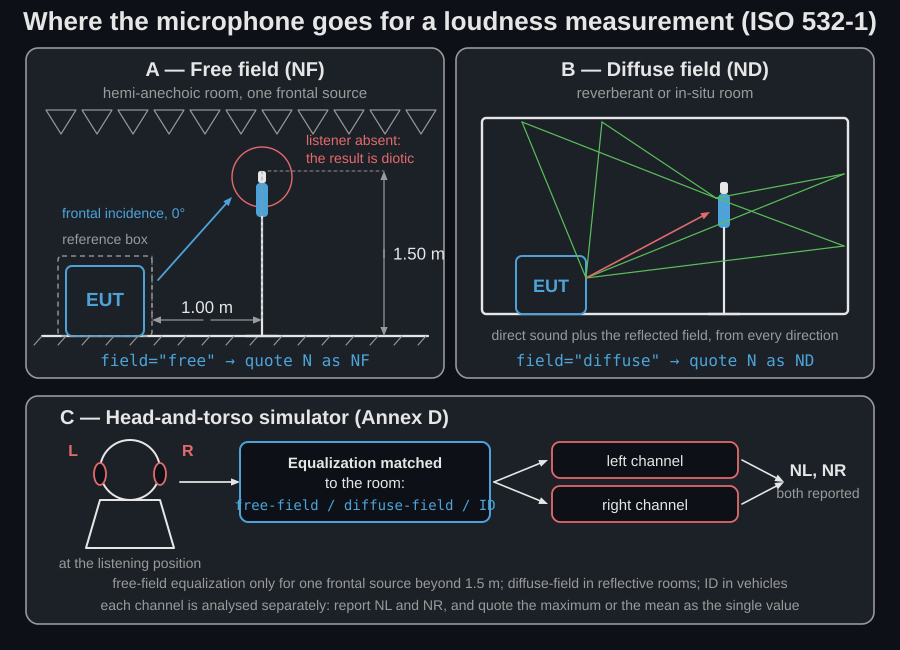
The three routes to a valid input. Panel A gives $N_F$ and panel B $N_D$; the field type is part of the result, not a preference.

Which field, and why it must be stated. field="free" applies the frontal free-field transfer of the head and outer ear and suits a direct field — anechoic room, close to a source, outdoors; field="diffuse" applies the random-incidence transfer and suits a reverberant room or an in-situ measurement. The correction is a fixed spectral shape applied to the band levels before the critical-band stage, largest above 1 kHz where head diffraction and ear-canal resonance differ most: on a flat 60 dB spectrum the diffuse-field result is 33.9 sone against 31.9 sone free field, 6 % — small beside a calibration error, large enough to matter when two products are being compared. Clause 4 requires the field type to be specified and clause 7 makes it part of the report, so “N = 13.1 sone” is incomplete: write $N_F$ or $N_D$, or say “free field” beside the number.

Artificial-head recordings. Annex D governs the head-and-torso route: the recording must already carry an equalization matched to the measuring environment — free-field only for a single frontal source beyond 1.5 m, diffuse-field in reflective surroundings, ID equalization in vehicles — and each ear channel is analysed separately, with both reported and the maximum or the mean quoted as the single value.

What the report has to contain (clause 7): the sound assessed, a reference to ISO 532-1, which method was used (stationary clause 5 or time-varying clause 6), the sound field F or D, the type of input data (band levels or time signal), the loudness in sones, and — for a time-varying run — the loudness time function, with $N_{\text{max}}$ and $N_5$ where required. ZwickerLoudness.report() prints the acoustic half of that list; the rest arrives through ReportMetadata.

import numpy as np
from phonometry import psychoacoustics

# A raw recording plus its calibration so the guide runs standalone
fs = 48000
x = 0.2 * np.sin(2 * np.pi * 1000 * np.arange(fs) / fs)   # any recording (digital units)
sens = 1.0                                                # calibration_factor to pascals
levels_28 = np.full(28, 60.0)                             # 28 one-third-octave band levels (dB)

# From a raw recording: calibration_factor scales digital units to Pa
res = psychoacoustics.loudness_zwicker(x, fs, field="free", calibration_factor=sens)
print(f"N = {res.loudness:.1f} sone  ({res.loudness_level:.0f} phon)")   # 13.1 sone (77 phon)

# Time-varying signals: percentile loudness N5 is the reporting standard.
# A 4.4 s train of 1 kHz bursts stepping 45 -> 85 dB, the loudest one brief.
segments = []
for level, seconds in [(45.0, 0.6), (55.0, 0.6), (65.0, 0.6), (75.0, 0.6), (85.0, 0.25)]:
    n = int(seconds * fs)
    k = np.arange(n)
    env = np.minimum(1.0, np.minimum(k, n - 1 - k) / (0.02 * fs))   # 20 ms ramps
    p = np.sqrt(2) * 2e-5 * 10 ** (level / 20)                      # peak amplitude (Pa)
    segments += [p * np.sin(2 * np.pi * 1000 * k / fs) * env, np.zeros(int(0.35 * fs))]
bursts = np.concatenate(segments)

tv = psychoacoustics.loudness_zwicker(bursts, fs)      # stationary=False (default)
print(f"{tv.n5:.1f} {tv.n10:.1f} {tv.loudness:.1f}")   # 14.5 11.4 22.5 — N5, N10, Nmax

# From 28 one-third-octave band levels (25 Hz .. 12.5 kHz)
res = psychoacoustics.loudness_zwicker_from_spectrum(levels_28, field="diffuse")

res.plot()   # N'(z) over the Bark scale — the specific-loudness pattern (needs matplotlib)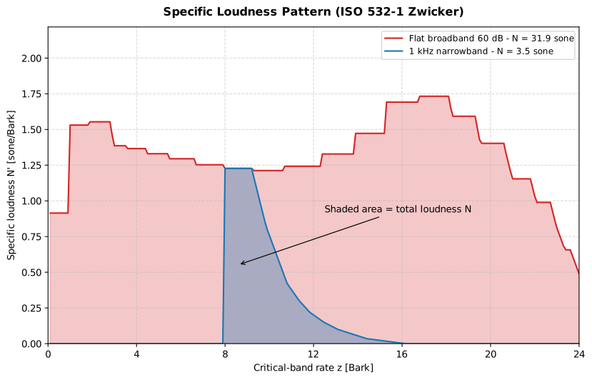

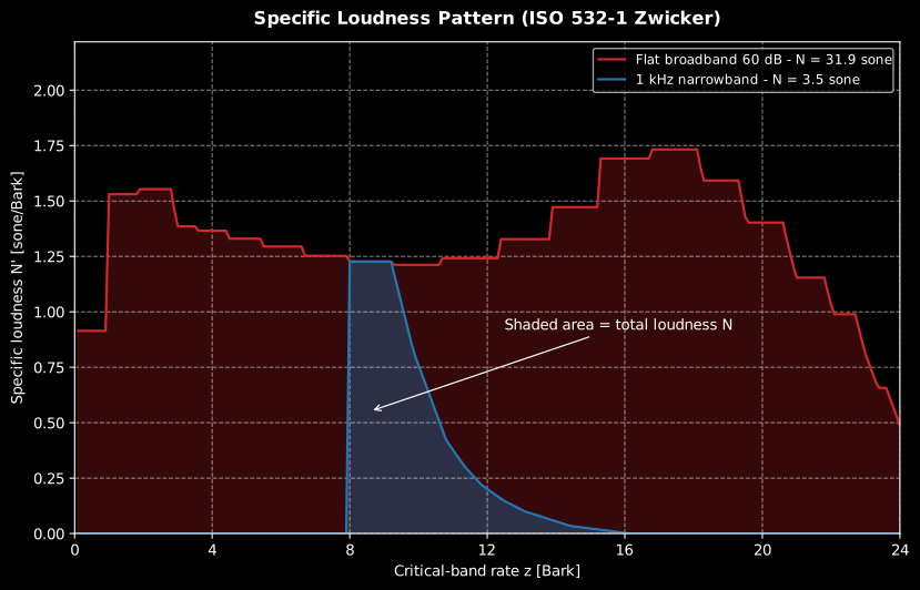
Same band level, very different loudness: energy spread over many critical bands (red) sums to far more sones than the same level concentrated in one band (blue). The area under $N^{\prime }(z)$ is the total loudness.

Show the code for this figure

import matplotlib.pyplot as plt
import numpy as np
from phonometry import psychoacoustics

levels_28 = np.full(28, 60.0)                             # 28 one-third-octave band levels (dB)
# From 28 one-third-octave band levels (25 Hz .. 12.5 kHz)
res = psychoacoustics.loudness_zwicker_from_spectrum(levels_28, field="diffuse")

# One line — the specific-loudness pattern N'(z) straight from the result:
res.plot()
plt.show()

# Or reproduce the figure by hand — two patterns of equal band level (60 dB),
# energy spread over many critical bands vs concentrated in the 1 kHz band:
narrow = psychoacoustics.loudness_zwicker_from_spectrum(np.r_[np.full(16, -60.0), 60.0, np.full(11, -60.0)])
broad = psychoacoustics.loudness_zwicker_from_spectrum(np.full(28, 60.0))
z = np.arange(1, narrow.specific.size + 1) * 0.1          # Bark axis
fig, ax = plt.subplots()
for r, color, label in [
    (broad, "#d62728", f"Flat broadband 60 dB - N = {broad.loudness:.1f} sone"),
    (narrow, "#1f77b4", f"1 kHz narrowband - N = {narrow.loudness:.1f} sone"),
]:
    ax.fill_between(z, r.specific, color=color, alpha=0.3)
    ax.plot(z, r.specific, color=color, label=label)
ax.set_xlabel("Critical-band rate z [Bark]")
ax.set_ylabel("Specific loudness N' [sone/Bark]")
ax.legend()
plt.show()

The implementation is a clean-room port of the standard’s normative reference program (Annex A.4): all twelve data tables are digit-exact and the full Annex B validation set runs in CI: the stationary test case reproduces the published value to every printed digit, and the tone-pulse $N(t)$ traces stay inside the standard’s per-sample 5 % tolerance band.

loudness_zwicker() parameters

Parameter	Type	Units	Range / default	Notes
x	1D array	Pa (after calibration)	≥ 8 ms at 48 kHz	Resampled internally to 48 kHz if needed
fs	int	Hz	> 0
field	str	—	'free' (default) / 'diffuse'	Sound-field correction (Table A.5)
stationary	bool	—	default False	True: single $N$ from the averaged spectrum
calibration_factor	float	Pa per digital unit	default 1.0	From sensitivity()

Returns a ZwickerLoudness dataclass: loudness_level (phon), specific ($N^{\prime }(z)$, 240 bins of 0.1 Bark), and for time-varying runs n5, n10, time and loudness_vs_time (500 Hz trace). loudness ($N$, sones) changes meaning with stationary: with stationary=True it is the single stationary $N$ of clause 5, and with the default stationary=False it is the peak $N_{\text{max}}$ of the clause 6 loudness-versus-time trace — which is why the first snippet above, run on a steady tone, already reports a maximum.

Reading a time-varying result (clause 6.4)

A fluctuating sound has no single loudness, so ISO 532-1 clause 6.4 reports a percentile: $N_5$, the loudness exceeded 5 % of the analysis time, because the arithmetic mean of $N(t)$ sits systematically below what listeners judge — on the burst train above the mean is 4.1 sone against $N_5=14.5$. $N_{10}$ is the gentler companion for sounds with brief peaks, and res.loudness is $N_{\text{max}}$: the right quantity for hunting the worst instant, the wrong one to quote as “the loudness”.

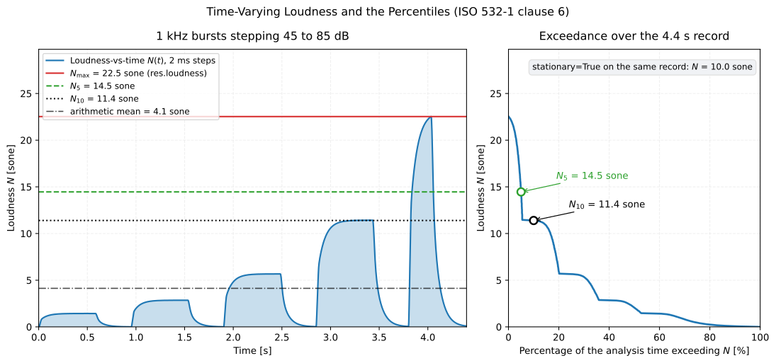
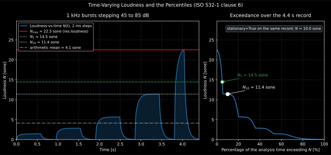
What a percentile of a loudness trace is. The brief 85 dB burst sets $N_{\text{max}}$ and almost nothing else: it occupies under 6 % of the record, so $N_5$ lands 8 sone below it. The same record analysed with stationary=True returns 10.0 sone, a fifth quantity again.

Show the code for this figure

import matplotlib.pyplot as plt

# `bursts` and `tv` come from the snippet above.
plt.plot(tv.time, tv.loudness_vs_time, label="N(t)")
for value, label in [(tv.loudness, "Nmax"), (tv.n5, "N5"), (tv.n10, "N10")]:
    plt.axhline(value, linestyle="--", label=f"{label} = {value:.1f} sone")
plt.xlabel("Time [s]")
plt.ylabel("Loudness N [sone]")
plt.legend()
plt.show()

Because $N_5$ is a percentage of the analysis window, lengthening or shortening the record moves it. Quote the measurement time beside $N_5$, keep it identical across the sounds being compared (clause 6.4 requires as much), and do not use $N_5$ for isolated impulses at all — that is exactly the case the trace above caricatures. loudness_vs_time and time carry the trace, so a record can be trimmed to the operating state of interest before the percentile is read, and the measurement interval belongs in ReportMetadata, since the fiche prints $N_5$ without one.

ISO 532-1 report (.report())

ZwickerLoudness.report(path) renders a one-page PDF fiche laid out like an accredited loudness report: a standard-basis line, an optional metadata header block, a compact metrics table (total loudness $N$, loudness level $L_N$, and the $N_5$/$N_{10}$ percentiles for a time-varying result) beside the specific-loudness pattern $N^{\prime }(z)$ (the result’s own .plot()), the boxed $N=X\text{sone}$ ($L_N=Y\text{phon}$) single number, an optional verdict row and a footer with the fixed disclaimer. It uses the same ReportMetadata container and rendering engine as the ISO 717 insulation fiche; a supplied requirement is read as the maximum permitted loudness in sone (a lower loudness passes). Rendering needs reportlab and, for the figure the fiche embeds, matplotlib (pip install "phonometry[report,plot]"); only engine="reportlab" is supported. The fiche renders in English by default; pass language="es" for a Spanish fiche (translated fixed strings and a comma decimal separator), e.g. res.report("loudness_fiche_es.pdf", language="es").

from phonometry import psychoacoustics, ReportMetadata

res = psychoacoustics.loudness_zwicker_from_spectrum(levels_28, field="free")
res.report(
    "loudness_fiche.pdf",
    metadata=ReportMetadata(
        specimen="Household appliance, steady operating noise",
        measurement_standard="ISO 532-1 method 1",
        laboratory="Phonometry Reference Laboratory",
        requirement=12.0,             # maximum permitted loudness (sone)
    ),
)                                     # N (sone) and LN (phon)

The example fiche is regenerated with make reports and kept rendered in the repository; click the preview to open the PDF.

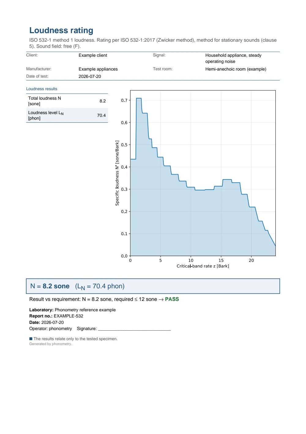
One-page loudness fiche: a metadata header, a metrics table with total loudness N and loudness level LN, the specific-loudness pattern over the critical-band rate, the boxed N = 8.2 sone (LN = 70.4 phon) single-number result and a PASS verdict against a 12 sone limit.

Download the report (PDF)

Zwicker loudness fiche (ZwickerLoudness.report), N in sone with LN in phon.

Loudness level of pure tones (ISO 226:2023)

The normal equal-loudness-level contours relate the SPL of a pure tone to its perceived loudness level in phons (the SPL of an equally loud 1 kHz tone). equal_loudness_contour(phon) evaluates ISO 226:2023 Formula (1) at the 29 preferred third-octave frequencies of Table 1, loudness_level(spl, frequency) is the exact inverse (Formula 2), and hearing_threshold() returns the threshold-of-hearing column. equal_loudness_contours(phons) bundles a whole family of contours with the threshold into a plottable EqualLoudnessContours result:

from phonometry import psychoacoustics

freqs, spl = psychoacoustics.equal_loudness_contour(40.0)   # the classic 40-phon contour
phon = psychoacoustics.loudness_level(73.0, 63.0)           # 73 dB @ 63 Hz -> 40 phon

# The whole family (20-90 phon by default) plus the hearing threshold:
res = psychoacoustics.equal_loudness_contours()
res.plot()   # the iconic ISO 226 chart (needs matplotlib)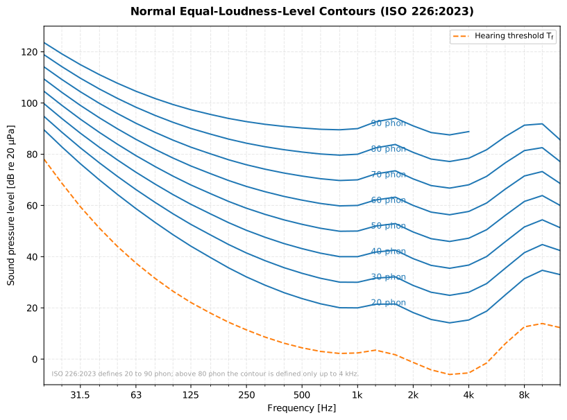

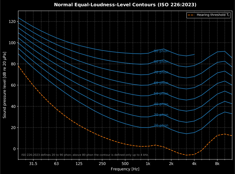
ISO 226:2023 defines the contours from 20 to 90 phon; above 80 phon the formula is valid only up to 4 kHz, so the 90 phon contour stops there and no higher contours are defined.

Show the code for this figure

import matplotlib.pyplot as plt
from phonometry import psychoacoustics

# One line — the contour family straight from the result:
res = psychoacoustics.equal_loudness_contours()
res.plot()
plt.show()

# Or reproduce the figure by hand — ISO 226:2023 Formula (1) at the 29
# preferred frequencies of Table 1, one contour per loudness level:
fig, ax = plt.subplots()
for phon in [20, 40, 60, 80, 90]:
    freqs, spl = psychoacoustics.equal_loudness_contour(float(phon))
    ax.semilogx(freqs, spl, color="C0")
    ax.annotate(f"{phon} phon", xy=(1000, phon + 1), fontsize=9)
ft, tf = psychoacoustics.hearing_threshold()
ax.semilogx(ft, tf, "--", color="C1", label="Hearing threshold $T_f$")
ax.set(xlabel="Frequency [Hz]", ylabel="Sound pressure level [dB re 20 µPa]")
ax.grid(True, which="both", alpha=0.3)
ax.legend()
plt.show()

Validity per clause 4.1: 20-90 phon (80 phon above 4 kHz); the implementation is verified against the Annex B tables in CI. Note this is the loudness of pure tones; the loudness of arbitrary signals in sones is what the ISO 532 models compute, the Zwicker method above and the newer families of Advanced Loudness.

Zwicker is the reference model, not the only one. The Moore-Glasberg loudness of ISO 532-2, its time-varying ISO 532-3 extension and the Sottek Hearing Model loudness of ECMA-418-2, together with the model-choice table that says when to prefer each, are Advanced Loudness.

What this guide covers

• Covered

  ISO 532-1:2017 (Zwicker method): the clause 4 input and instrumentation requirements, the stationary method of clause 5 and the time-varying method of clause 6 with the clause 6.4 percentile rules, ported from the normative Annex A.4 reference program and validated against Annex B, with the n5/n10 percentiles, via loudness_zwicker() and loudness_zwicker_from_spectrum(); the clause 7 reporting list and the Annex D guidance for head-and-torso recordings. ISO 226:2023: Formula (1), Formula (2) and the Table 1 contour parameters, via equal_loudness_contour(), loudness_level(), hearing_threshold() and equal_loudness_contours().

• Not covered

  The Moore-Glasberg loudness of ISO 532-2, the time-varying ISO 532-3 method and the Sottek Hearing Model loudness of ECMA-418-2 have moved to Advanced Loudness. The ISO 226:2023 contours describe pure tones only, and the standard defines no interpolation between the 29 tabulated frequencies, so loudness_level() expects one of the Table 1 frequencies.

See also

• Advanced Loudness (ISO 532-2/-3, ECMA-418-2): the Moore-Glasberg and Sottek loudness models and the model-choice table.
• Sound Quality Metrics: sharpness, tonality and roughness, the other half of the sound-quality story.
• Psychoacoustic annoyance and fluctuation strength: the Zwicker and Fastl model that consumes the percentile loudness $N_5$.
• Theory: the equations behind the loudness models.
• API reference: psychoacoustics.loudness.zwicker and psychoacoustics.loudness.contours.
• Theory: Zwicker loudness (ISO 532-1): the specific-loudness integral of ISO 532-1 and the excitation pattern it runs over.

Quick answers

What is the difference between loudness in sones and loudness level in phons?

Loudness $N$ in sones (ISO 532-1) is a ratio scale of perceived loudness: 4 sones is twice as loud as 2 sones, and by definition a 1 kHz tone at 40 dB SPL is 1 sone. Loudness level in phons (ISO 226) is the SPL of an equally loud 1 kHz pure tone, and every +10 phon doubles the sone value.

Over what range are the ISO 226:2023 equal-loudness contours valid?

ISO 226:2023 clause 4.1 defines the normal equal-loudness-level contours from 20 to 90 phon, evaluated at the 29 preferred third-octave frequencies of Table 1; above 80 phon the formula is valid only up to 4 kHz, so the 90 phon contour stops there and no higher contours are defined. The contours describe pure tones, not arbitrary signals.

References

• Fastl, H., & Zwicker, E. (2007). Psychoacoustics: Facts and models (3rd ed.). Springer. https://doi.org/10.1007/978-3-540-68888-4The critical-band and masking psychoacoustics behind the Zwicker model.
• Fletcher, H., & Munson, W. A. (1933). Loudness, its definition, measurement and calculation. The Journal of the Acoustical Society of America, 5(2), 82-108. https://doi.org/10.1121/1.1915637The original equal-loudness measurements behind the loudness-level concept of the pure-tone section.
• International Organization for Standardization. (2017). Acoustics — Methods for calculating loudness — Part 1: Zwicker method (ISO 532-1:2017). Stationary and time-varying loudness in sones from the normative Annex A.4 reference program, with the N5/N10 percentile loudness, validated against the Annex B set.
• International Organization for Standardization. (2023). Acoustics — Normal equal-loudness-level contours (ISO 226:2023). The contour model and Table 1 parameters behind the pure-tone loudness levels: the contours (Formula 1), the loudness level of pure tones (Formula 2) and the hearing threshold.