Noise-induced hearing loss (ISO 1999)
Standards: ISO 1999DHHS/NIOSH Publication No. 98-126Key references: Passchier-Vermeer 1974
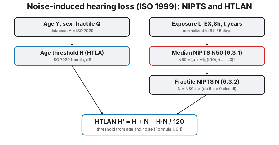
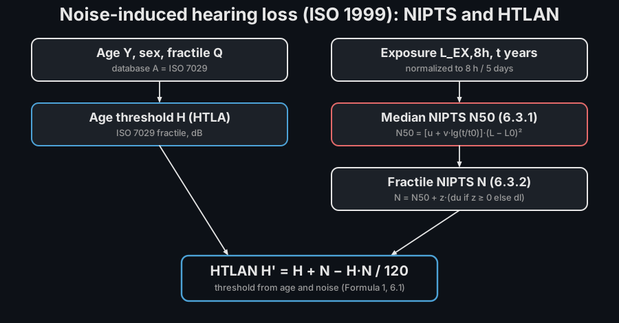
ISO 1999:2013 estimates the hearing loss a population suffers from occupational noise. It gives the noise-induced permanent threshold shift (NIPTS), the extra hearing loss caused by the noise, on top of ageing, as a function of the exposure level, the exposure duration and the audiometric frequency, together with its spread across a population. It then combines the noise component with the age component (the ISO 7029 threshold, “database A”) into the hearing threshold level associated with age and noise (HTLAN). Both are defined at the six audiometric frequencies 500 Hz to 6000 Hz, where noise damage concentrates (the characteristic 4 kHz notch).
1. Noise-induced permanent threshold shift (clause 6.3)
Section titled “1. Noise-induced permanent threshold shift (clause 6.3)”The median NIPTS for exposure durations of 10 to 40 years grows with the square of the excess of the noise exposure level over a frequency-dependent cut-off (ISO 1999 clause 6.3.1, Formula 2, Table 1):
with the exposure in years and year; below the effect is zero. A population fractile follows from two half-Gaussians whose spreads (worse than the median) and (better) are given by Formulae 6/7 and Table 3: with the standard-normal quantile, clamped at zero (clause 6.3.2).
The fractile argument is the fraction of the population below the returned
value, so fractile=0.9 is the most-susceptible tenth. Note that ISO 1999
writes its own percentage the other way round: in Formulae (4)/(5) is
the percentage with worse hearing, so that same tenth is , which
is how the .report() fiche prints it and how the Annex D columns are headed.
from phonometry import hearing
# Median NIPTS after 20 years at an 8 h-normalised level of 90 dB(A).r = hearing.nipts(90.0, 20.0, fractile=0.5)print(r.frequencies.astype(int))  # [ 500 1000 2000 3000 4000 6000]print(r.median.round(1))          # [ 0.   0.1  4.1 10.2 12.9  8.5]
# The most-susceptible tenth of the population (90th percentile):print(hearing.nipts(90.0, 20.0, fractile=0.9).value.round(1))# [ 0.   0.1  7.7 16.2 17.8 13.6]
r.plot()   # the NIPTS spectrum with its fractile band (needs matplotlib)
The shift peaks near 4 kHz and deepens with both level and duration. Below the
cut-off (here 500 Hz, dB, and 1000 Hz, dB, at 90 dB)
the noise causes no permanent shift. For durations under 10 years the median is
extrapolated from the 10-year value (Formula 3); a subset of the frequencies
can be requested with frequencies=.
What must be. The first argument is the A-weighted noise exposure level normalised to a nominal eight-hour day, in practice the result of an ISO 9612 survey of the homogeneous exposure group, which is the standard ISO 1999 references normatively for it. It is the level at the unprotected ear: the Scope says in as many words that none of its levels account for hearing protectors, which would both reduce the effective exposure and change the spectrum at the ear, so feeding an attenuated or “effective” level is not a conservative shortcut but a different quantity. Report the protector separately. The model also treats the level as constant over the whole duration, so a career of changing jobs is split into segments and each predicted on its own level rather than averaged first: Formula (2) is quadratic in the excess over , so averaging before squaring under-predicts. And the duration is exposure years, not age and not years of employment.
The level is also the variable a hearing-conservation decision acts on, and it is the one the two figures on this page hold fixed:
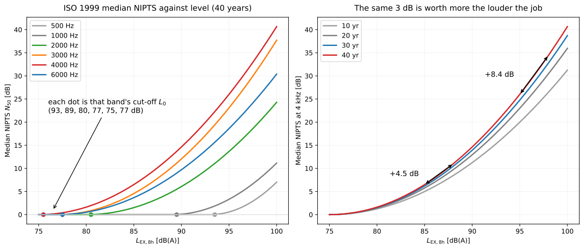
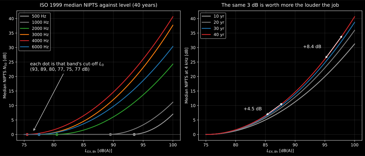
Below its cut-off the model returns exactly zero, and above it the shift is quadratic in the excess, so equal decibel reductions are worth progressively more the louder the job. On the right, at 4 kHz over a 40-year career, taking 3 dB off an 88 dB(A) job recovers 4.5 dB of median shift, while taking the same 3 dB off a 98 dB(A) job recovers 8.4 dB. That asymmetry, not the notch shape, is what a control measure is bought against.
Show the code for this figure
import matplotlib.pyplot as pltimport numpy as np
# `hearing` and the result `r` come from the first snippet on this page.levels = np.arange(75.0, 100.5, 0.5)fig, (ax_f, ax_t) = plt.subplots(1, 2, figsize=(12.5, 5.4))for k, f in enumerate(r.frequencies):    ax_f.plot(levels, [hearing.nipts(x, 40.0, 0.5).median[k] for x in levels],              label=f"{f:g} Hz")ax_f.legend()
for years in (10, 20, 30, 40):    ax_t.plot(levels, [hearing.nipts(x, years, 0.5).median[4] for x in levels],              label=f"{years} yr")     # index 4 is 4000 Hzax_t.legend()plt.show()
A longer, louder career makes the shape unmistakable:
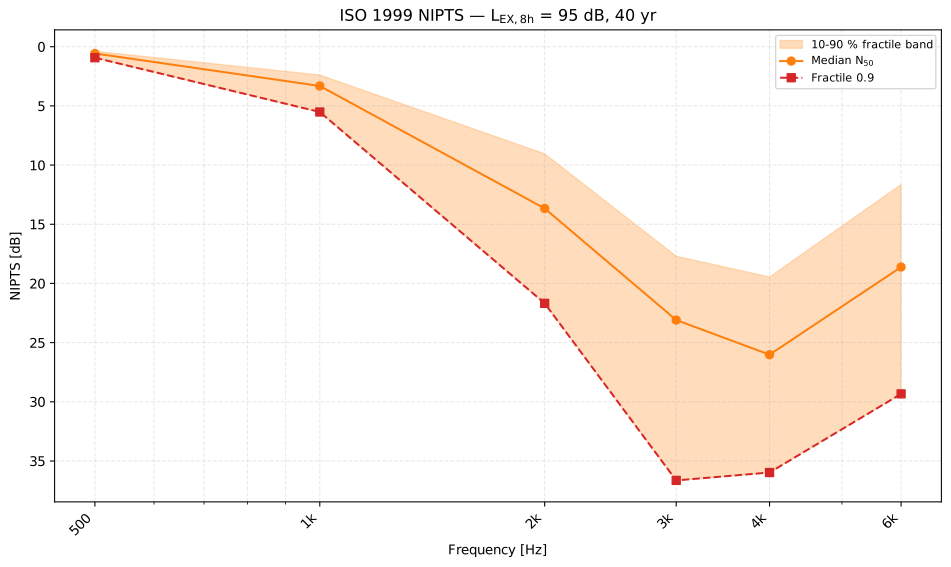
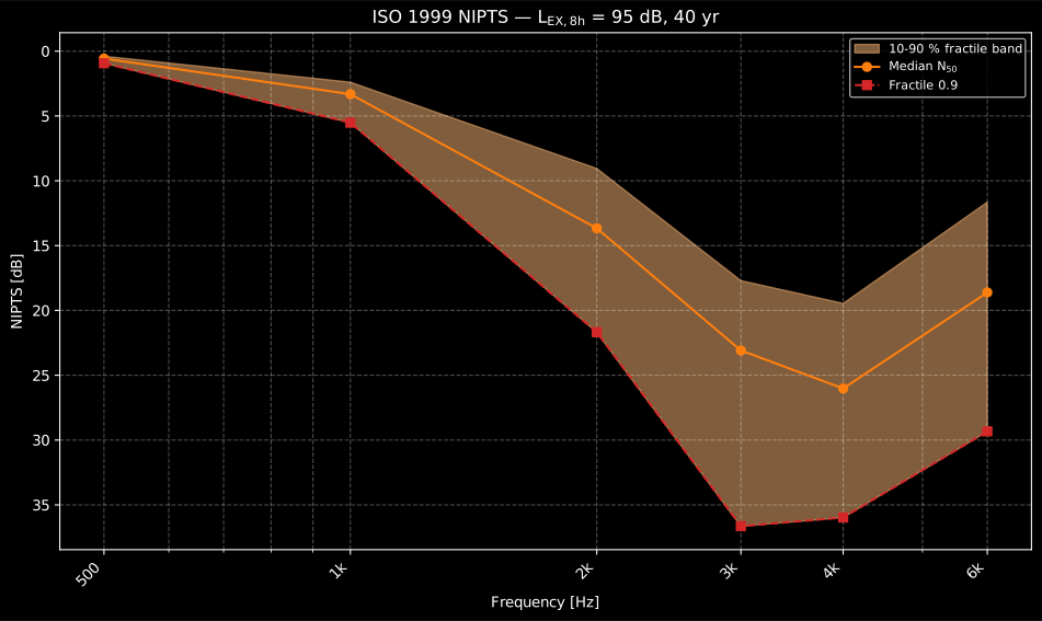
Show the code for this figure
import matplotlib.pyplot as pltfrom phonometry import hearing
# 40 years at an 8 h-normalised 95 dB(A), most-susceptible tenth.res = hearing.nipts(95.0, 40.0, fractile=0.9)print(res.median.round(1))    # the median N50print(res.value.round(1))     # the 90 % fractile
# One line: the median, the fractile and the 10-90 % band.res.plot()plt.show()
The notch at 3 kHz to 4 kHz, with partial recovery at 6 kHz, is the signature of noise damage and the reason audiometric surveillance tests those frequencies. It comes out of the model rather than being imposed on it: the cut-off level and the coefficients , of Table 1 are lowest where the ear is most vulnerable, so the same buys far more shift at 4 kHz than at 500 Hz.
Where the model applies
Section titled “Where the model applies”Formula (2) is a quadratic with no upper bound, so it keeps returning
plausible-looking numbers well outside the data that fitted it. Four limits
matter, and the library says so at three of them by raising
NoiseInducedHearingLossWarning:
- Duration. The median is specified for 10 to 40 years, with Formula (3) extrapolating down to 1 year. A six-month exposure or a fifty-year career is outside the fitted range and warns.
- Level. The Annex D worked examples span 85 dB to 100 dB, and Scope NOTE 4 restricts validity to the stated ranges of levels; above 100 dB the guide warns, and use above 200 Pa (140 dB) is recognised as extrapolation by the Scope itself.
- Fractile. Clause 6.3.2 calls the tails below = 5 % and above 95 % unreliable and says they should not be estimated, so the 0.9 / 0.1 pair used in the examples above already sits close to the practical edge, and anything beyond warns.
- The character of the noise. This one is silent, because no argument carries it. Scope NOTE 3 says the prediction method is based primarily on data collected with essentially broadband, steady, non-tonal noise, and the Scope covers noise below roughly 10 kHz that is steady, intermittent, fluctuating or irregular. An impulsive or strongly tonal exposure is therefore a use outside the evidence rather than a computation error, and the Introduction sets blast and high-impulse noise apart explicitly. NOTE 4 adds a second silent limit: the simplifications behind the data assume a daily exposure duration no longer than 12 h.
NIPTS report (.report())
Section titled “NIPTS report (.report())”NiptsResult.report(path) renders a one-page PDF fiche laid out like the
noise-induced hearing loss prediction an occupational-hygiene service issues
for an exposure group, following ISO 1999:2013 (clause 6.3): a
prediction-basis line, an optional metadata header block (company,
worker(s)/group, workplace and date of assessment), a table of the median
and the fractile NIPTS at the six audiometric frequencies beside the
result’s own spectrum plot with its fractile band, the boxed shift averaged
over the 2/3/4 kHz hearing-handicap set together with the exposure conditions
(, the duration in years and the population percentage ), and the
notes that keep the fiche honest: the values are a statistical prediction for
the exposed population rather than anyone’s audiogram, and ISO 1999 leaves the
choice of handicap frequencies to the user. verbose=True adds the spread
columns /; a requirement in the metadata is read as the maximum
acceptable representative NIPTS and adds a PASS/FAIL row (a smaller shift
passes). Rendering needs reportlab and matplotlib
(pip install "phonometry[report,plot]"); only engine="reportlab" is
supported, and language="es" renders a Spanish fiche.
from phonometry import hearing, ReportMetadata
# The 90 dB(A) / 20 year case above, most-susceptible tenth.res = hearing.nipts(90.0, 20.0, fractile=0.9)res.report(    "nipts_fiche.pdf",    metadata=ReportMetadata(        client="Example fabrication works",        specimen="Welders (homogeneous exposure group, 4 workers)",        test_room="Steel assembly hall, line 2",    ),)                                   # NIPTS averaged over 2/3/4 kHz (dB)
The example fiche is regenerated with make reports and kept rendered in the
repository; click the preview to open the PDF.
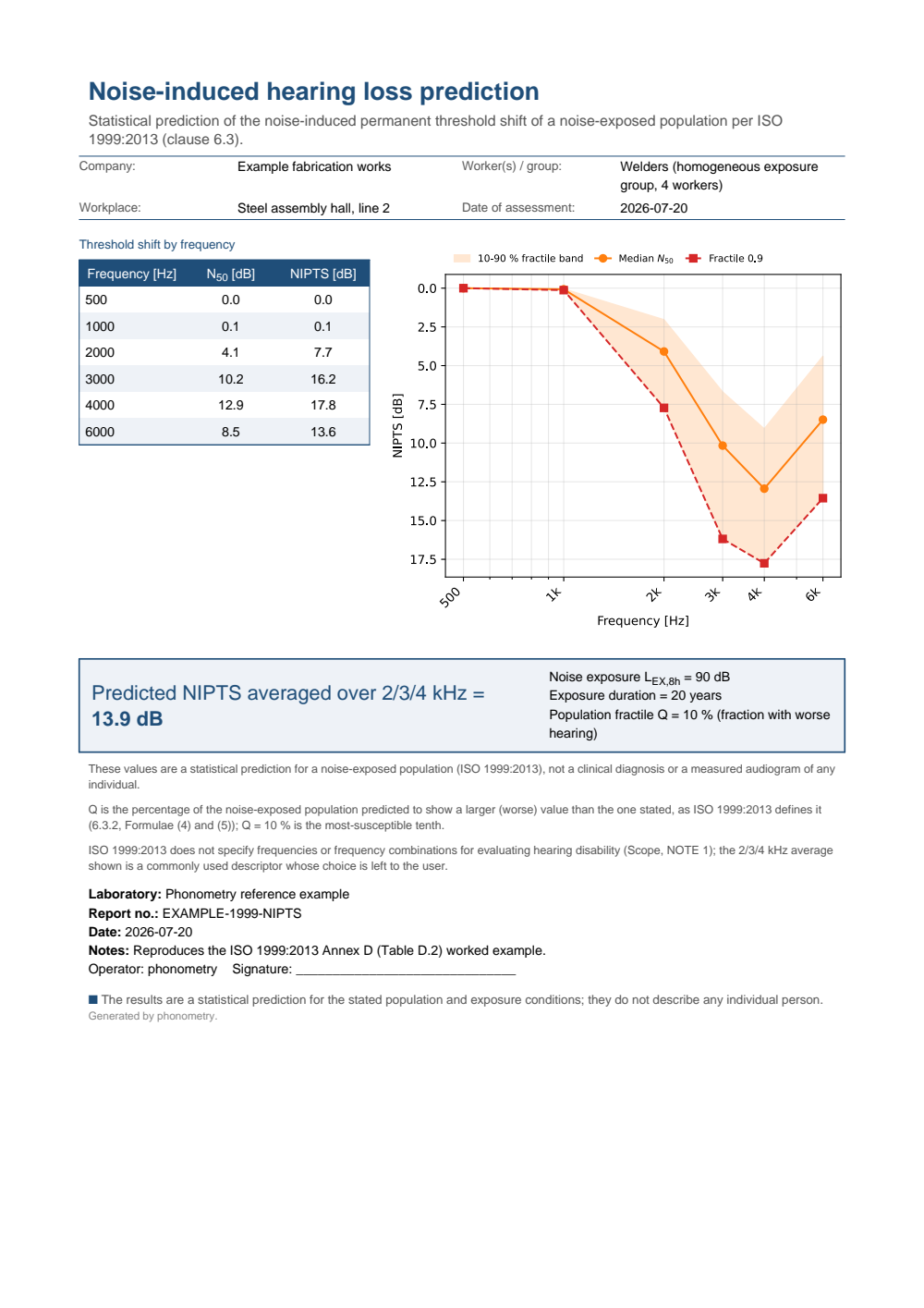
One-page noise-induced hearing loss prediction fiche: a metadata header (company, worker group, workplace, date of assessment), a table of the median N50 and the NIPTS at the requested fractile from 500 Hz to 6000 Hz (12.9 dB and 17.8 dB at 4000 Hz), the spectrum plot with its 10-90 % fractile band, and the boxed predicted NIPTS averaged over 2/3/4 kHz = 13.9 dB for a noise exposure LEX,8h = 90 dB over 20 years at population fractile Q = 10 %.
2. Age and noise combined: HTLAN (clause 6.1)
Section titled “2. Age and noise combined: HTLAN (clause 6.1)”The noise component does not simply add to the age component: ISO 1999 Formula (1) combines them with a compression term that matters once the total exceeds about 40 dB:
where is the age threshold (HTLA, from ISO 7029 at the same fractile) and
the NIPTS. htlan evaluates both components and their combination.
from phonometry import hearing
# A 60-year-old man, 30 years at 95 dB(A), median.h = hearing.htlan(60, "male", 95.0, 30.0, fractile=0.5)print(h.htla.round(1))       # [ 6.   7.8 12.5 16.6 20.2 25.9]  age aloneprint(h.nipts.round(1))      # [ 0.5  3.  11.8 21.6 24.8 17.6]  noise aloneprint(h.threshold.round(1))  # [ 6.5 10.7 23.  35.2 40.8 39.8]  age + noise
h.plot()   # the three curves of the figure below: HTLA, NIPTS and HTLAN
At 4 kHz the age component (20.2 dB) and the noise component (24.8 dB) combine to 40.8 dB rather than their 45.0 dB sum; the compression term removes 4.2 dB.
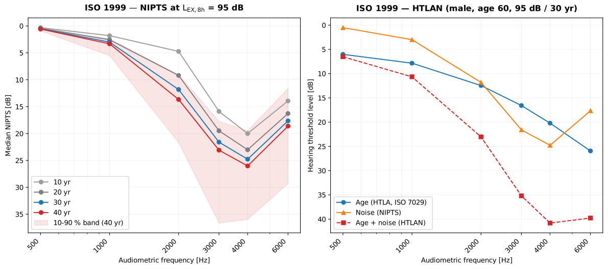
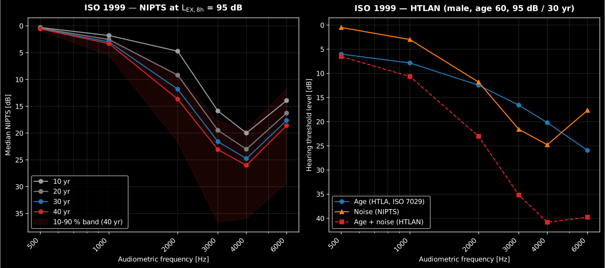
Show the code for this figure
import matplotlib.pyplot as pltfrom phonometry import hearingfrom phonometry.hearing.noise_induced_hearing_loss import NIPTS_FREQUENCIES as f
# One line for the NIPTS spectrum with its fractile band:hearing.nipts(95.0, 40.0, 0.9).plot()plt.show()
# By hand, both panels:fig, (ax1, ax2) = plt.subplots(1, 2, figsize=(12.5, 5.6))for yr in (10, 20, 30, 40):    ax1.plot(f, hearing.nipts(95.0, yr, 0.5).median, "o-", label=f"{yr} yr")ax1.set_xscale("log"); ax1.invert_yaxis(); ax1.legend()
h = hearing.htlan(60, "male", 95.0, 30.0, 0.5)ax2.plot(f, h.htla, "o-", label="Age (HTLA)")ax2.plot(f, h.nipts, "^-", label="Noise (NIPTS)")ax2.plot(f, h.threshold, "s--", label="Age + noise (HTLAN)")ax2.set_xscale("log"); ax2.invert_yaxis(); ax2.legend()plt.show()
Three quantities, kept distinct. It is worth being precise about what each symbol means, because they are easy to conflate:
- NIPTS () is the noise-induced permanent threshold shift: the extra loss the noise causes, and nothing else. It is what an ideal hearing- conservation programme would prevent. On its own it is not an audiogram.
- HTLA () is the age threshold alone (the ISO 7029 component of the hearing-threshold guide), the loss the same person would have with no occupational noise.
- HTLAN () is the total threshold: age and noise combined by Formula (1). This is what an audiometer measures, and the only one of the three you can compare against a real audiogram.
The non-linear combination is why you cannot simply read NIPTS off a measured audiogram by subtracting an age table: near-total losses would otherwise exceed the ~120 dB physiological ceiling, so the standard compresses the sum. Because the correction scales with the product of the two components, it can already shave a few dB while is below 40 dB; 40 dB is only a rough marker for where the effect becomes noticeable, not a hard boundary, and the correction grows steadily in the regime of a long, loud exposure where both terms are large.
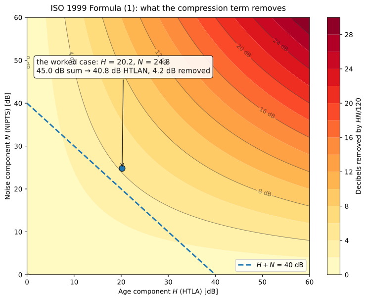
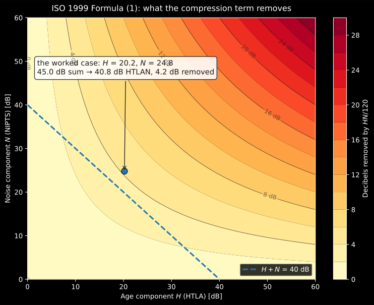
The correction is a product, so it has no threshold: the dashed dB line cuts across the contours instead of following one. A large age component makes a modest noise component compress, and the other way round: 4.2 dB is already gone at the worked case, and a worker with 40 dB from each cause loses 13.3 dB from the sum.
Show the code for this figure
import matplotlib.pyplot as pltimport numpy as np
# `hearing` is the import of the first snippet on this page.grid = np.linspace(0.0, 60.0, 121)h, n = np.meshgrid(grid, grid)removed = h + n - hearing.combine_age_and_noise(h, n)print(round(float(removed[-1, -1]), 1))          # 30.0 dB at H = N = 60
fig, ax = plt.subplots(figsize=(8.2, 6.4))cs = ax.contourf(h, n, removed, levels=np.arange(0.0, 31.0, 2.0), cmap="YlOrRd")fig.colorbar(cs, ax=ax)ax.plot([0.0, 40.0], [40.0, 0.0], "--")          # H + N = 40 dBplt.show()
Comparing with a measured audiogram
Section titled “Comparing with a measured audiogram”HTLAN is comparable only with an audiogram taken the way the underlying databases were taken, and ISO 1999 makes the technique part of the comparison rather than an implementation detail: clause 6.2.3 states that because audiometric measurement techniques affect threshold measurements, the same technique should be used to establish the HTLA database as is used to obtain or verify the threshold of the noise-exposed population. Change the earphone or the threshold procedure and the offset between measured and predicted moves. In practice that means:
- Pure-tone air conduction. Annex A.1 says database A is the ISO 7029 distribution of the normal threshold of hearing by air conduction, so a bone conduction threshold is not the quantity being predicted.
- A declared, calibrated earphone. dB HL is transducer-specific: 0 dB HL is the reference equivalent threshold sound pressure level of ISO 389-1 (supra-aural), ISO 389-2 (insert) or ISO 389-8 (circumaural) for the earphone actually fitted. Record which, and its calibration.
- A stated threshold procedure. ISO 8253-1:2010 clause 6.2.3 specifies two manual procedures, ascending and bracketing, which differ only in the sequence of presentations and, properly carried out, give substantially the same thresholds. Record which one, and note that a procedure outside that clause can move the threshold by several decibels on average.
- The same six frequencies.
niptsandhtlanreturn 500, 1000, 2000, 3000, 4000 and 6000 Hz. An audiogram that omits 3 kHz or 6 kHz cannot be compared where the noise notch lives. - A fixed ear convention. Worse ear, better ear or the two-ear average are three different comparisons against the same prediction, and ISO 1999 leaves the choice to the user, so it belongs in the report rather than in the analyst’s head.
- A noise-free interval before the test. NIPTS is permanent shift, and it is preceded by a reversible temporary threshold shift; ISO 8253-1 clause 5.1 says significant noise exposure before audiometry shall be avoided or else noted. A mid-shift audiogram measures TTS on top of the permanent loss and will exceed the predicted HTLAN for a reason the model does not describe. Record the elapsed time since the last exposure.
One caution that applies to the whole comparison: the Scope states that the standard is based on statistical data and cannot be applied to the prediction or assessment of an individual’s hearing loss except in terms of statistical probabilities. A single audiogram sitting above the median is not evidence of anything; a distribution of audiograms sitting above the predicted fractiles is.
Fence caveats. ISO 1999 gives thresholds and their distribution; it does not define a “hearing handicap” or a compensable fence. A fence is a policy line (commonly a 25 dB average over selected frequencies) above which hearing is deemed impaired, and it lives in national regulation, not in this standard. Two cautions follow. First, the fence frequencies matter: averaging over 0.5/1/2 kHz (a classic speech fence) barely sees the 3–6 kHz noise notch, so it under-reports early noise damage that a 3/4/6 kHz average would catch. Second, NIPTS and HTLAN answer different fence questions: NIPTS asks “how much did the noise add”, HTLAN “is this ear, age included, over the line”; and a population’s percentage beyond fence depends on the fractile spread, not just the median, so it must be read from the distribution, never from the median threshold alone.
The NiptsResult carries the median (), the
spread_upper/spread_lower
and the value at the requested fractile; the HtlanResult carries htla,
nipts and the combined threshold. Both expose .plot(). The age component
alone is the subject of the
hearing-threshold guide.
HTLAN report (.report())
Section titled “HTLAN report (.report())”HtlanResult.report(path) renders the companion fiche for the combined
threshold, following ISO 1999:2013 clause 6.1: the same prediction-basis
line and metadata header as the NIPTS fiche, but a table that carries the age
component , the noise component and the combined at each
audiometric frequency, beside the three-curve plot, with the boxed threshold
averaged over the 2/3/4 kHz hearing-handicap set and the listener and exposure
conditions (age and sex, over the exposure years, and the
population percentage ). Its notes add the one that matters here: the age
component is database A evaluated from ISO 7029:2017, whose values differ from
the illustrative Table A.3 selection of ISO 1999, which derives from an earlier
edition. verbose=True adds the compression term as its own column,
and a requirement in the metadata is read as the maximum acceptable
representative HTLAN.
from phonometry import hearing, ReportMetadata
# The 60-year-old machine operator of this section, median.res = hearing.htlan(60, "male", 95.0, 30.0, fractile=0.5)res.report(    "htlan_fiche.pdf",    metadata=ReportMetadata(        client="Example fabrication works",        specimen="Machine operator (60 years, 30 years in role)",        test_room="Steel assembly hall, line 2",    ),)                                   # HTLAN averaged over 2/3/4 kHz (dB HL)
The example fiche is regenerated with make reports and kept rendered in the
repository; click the preview to open the PDF.
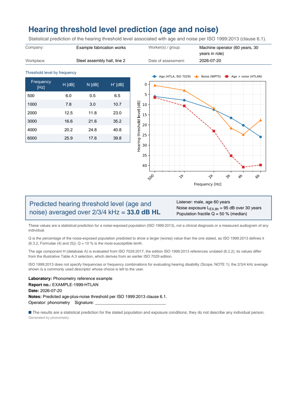
One-page hearing threshold level prediction fiche for age and noise: a metadata header, a table of the age component H, the noise component N and the combined threshold H' from 500 Hz to 6000 Hz (20.2, 24.8 and 40.8 dB at 4000 Hz), the plot of the three curves, and the boxed predicted hearing threshold level averaged over 2/3/4 kHz = 33.0 dB HL for a 60-year-old male listener exposed at LEX,8h = 95 dB over 30 years at population fractile Q = 50 %.
What this guide covers
Section titled “What this guide covers”Covered
ISO 1999:2013 as implemented by
niptsandhtlan: the median NIPTS of clause 6.3.1 (Formula 2, extrapolated below 10 years by Formula 3, Table 1) and its population fractile of clause 6.3.2 (Formulae 4-7, Tables 2-3), together with the HTLAN combination of clause 6.1 (Formula 1) run bycombine_age_and_noise, all validated against the Annex D worked examples. The age component is database A, evaluated from ISO 7029:2017, the edition clause 6.2.2 references undated.Not covered
Clauses 6.2.3 and 6.2.4 let the user substitute a database B for database A: an age threshold measured on a control population of the country under consideration. Only database A is implemented, so
htlanalways draws its age component from ISO 7029:2017.combine_age_and_noiseaccepts an external HTLA array for that case, but computing database B itself is not phonometry’s job. ISO 1999 does not define a “hearing handicap” or a compensable fence: that line is set by national regulation, and nothing here applies one, so you must supply and check it yourself.
References
Section titled “References”- International Organization for Standardization. (2013). Acoustics — Estimation of noise-induced hearing loss (ISO 1999:2013). The implemented model: the HTLAN combination (clause 6.1, Formula 1), the median NIPTS (clause 6.3.1, Formulae 2-3, Table 1) and its statistical distribution (clause 6.3.2, Formulae 4-7, Tables 2-3), validated against the worked examples of Annex D. The age component (database A) is ISO 7029:2017.
- National Institute for Occupational Safety and Health. (1998). Criteria for a recommended standard: Occupational noise exposure — Revised criteria 1998 (DHHS/NIOSH Publication No. 98-126). https://doi.org/10.26616/NIOSHPUB98126A freely available criteria document (the linked PDF is the free download) reviewing the same exposure-response evidence and the fence and hearing-conservation issues discussed on this page.
- Passchier-Vermeer, W. (1974). Hearing loss due to continuous exposure to steady-state broad-band noise. The Journal of the Acoustical Society of America, 56(5), 1585-1593. https://doi.org/10.1121/1.1903482One of the field studies whose exposure-response data underpin the NIPTS relations later codified in ISO 1999.