Objective audibility of tones in noise (ISO/PAS 20065)

A steady tone embedded in broadband noise stands out when it rises audibly above the noise that would otherwise mask it, the objective precondition for the tonal penalties applied in noise assessment. ISO/PAS 20065:2016 is the engineering method that quantifies this audibility: from a narrow-band FFT spectrum it derives, for every prominent tone, the audibility $\Delta L$: how many decibels the tone level exceeds the masking threshold of the surrounding noise. It is the detailed method that ISO 1996-2:2017 defers to (the simpler Annex C route lives in environmental measurement); the mean audibility $\Delta L$ it produces feeds the ISO 1996-2 tonal adjustment $K_t$.

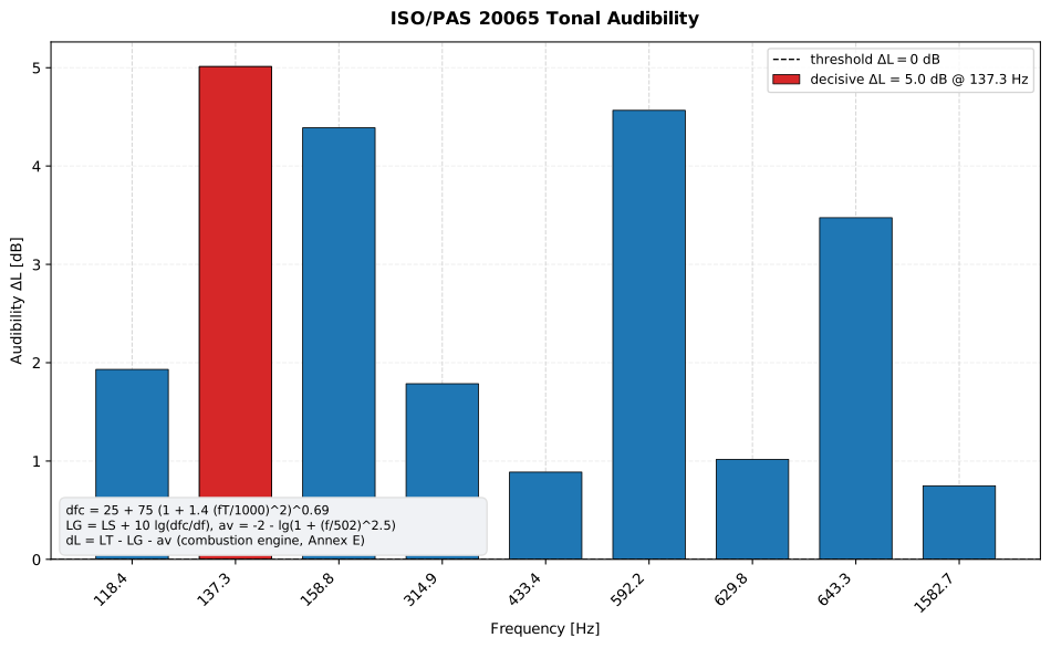
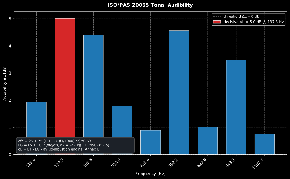
The nine tones of the ISO/PAS 20065 Annex E combustion-engine spectrum, each evaluated in its own critical band. A bar above the dashed $\Delta L=0$ dB line is audible over the masking noise around it, and the tallest of them — the 137.3 Hz tone at 5.0 dB — is the largest per-tone audibility of this spectrum. It is not yet the spectrum’s decisive audibility: §3 shows why the standard’s own answer is 9.18 dB.

Show the code for this figure

import matplotlib.pyplot as plt
from phonometry import psychoacoustics

# ISO/PAS 20065 Annex E combustion-engine spectrum 1: nine tones (fT, LT, LS)
# from a narrow-band spectrum with line spacing 2.7 Hz
fT = [118.4, 137.3, 158.8, 314.9, 433.4, 592.2, 629.8, 643.3, 1582.7]
LT = [64.56, 67.96, 68.63, 68.50, 73.17, 78.31, 75.00, 79.75, 71.07]
LS = [48.91, 49.22, 50.50, 52.85, 58.29, 59.53, 59.71, 61.98, 54.16]

res = psychoacoustics.assess_tones(fT, LT, LS, 2.7)
print(round(res.decisive_audibility, 2), res.decisive_frequency)  # 5.01 137.3
res.plot()   # per-tone audibility bars, decisive tone highlighted
plt.show()

0. The spectrum this method needs

Every later section consumes a narrow-band spectrum, and ISO/PAS 20065 is specific about which one. A reader can follow this page end to end and produce an audibility the standard would reject, because the analyser was set up differently: the arithmetic gives no sign of it.

Analyser settings (clause 4.2). A class 1 chain per IEC 61672-1 with a lower limiting frequency at or below 20 Hz, an anti-aliasing filter ahead of the digitisation, and an amplitude resolution of at least 0.1 dB. The constant line spacing $\Delta f$ shall lie between 1.9 Hz and 4.0 Hz inclusive — the 2.7 Hz of the Annex E example sits in the middle of that window, which is what assess_tones(..., 2.7) carries as its last argument. The Hanning window is mandatory, and it is where the −1.76 dB bandwidth correction of §2 comes from: another window has another effective bandwidth, so that constant, and with it every level in the chain, would be wrong.

A-weighting, before anything else (clause 5.3.2). The method is defined on an A-weighted narrow-band spectrum; the library is weighting-agnostic and applies nothing, so the caller weights the lines first. It matters because the audibility is a difference of two levels taken over one critical band: a weighting flat across the band would cancel out, but the A-curve is steepest exactly where tonal complaints live. At the 137.3 Hz tone of the example it is about −15 dB, and it climbs nearly 9 dB across that tone’s own critical band (−19.8 dB at 95.7 Hz to −11.0 dB at 197.0 Hz), so both $L_T$ and $L_S$ move, and by different amounts. The Annex E numbers on this page are already A-weighted, which is the tell-tale: anyone reproducing them from an unweighted analyser will find low-frequency tones reading high.

Averaging (clauses 4.3 and 5.1). The analyser’s own basic spectra are shorter than a second at this line spacing, so they are merged line by line (Formula 1) into spectra of approximately 3 s. That 3 s is a floor, not a preference: clause 5.1 states that shorter averaging yields unjustified audibilities, too high and too low. At least 12 time-staggered 3 s spectra are then taken, because that is what generally keeps the extended uncertainty inside ±1.5 dB, and every alternating operating state of the source must appear among them.

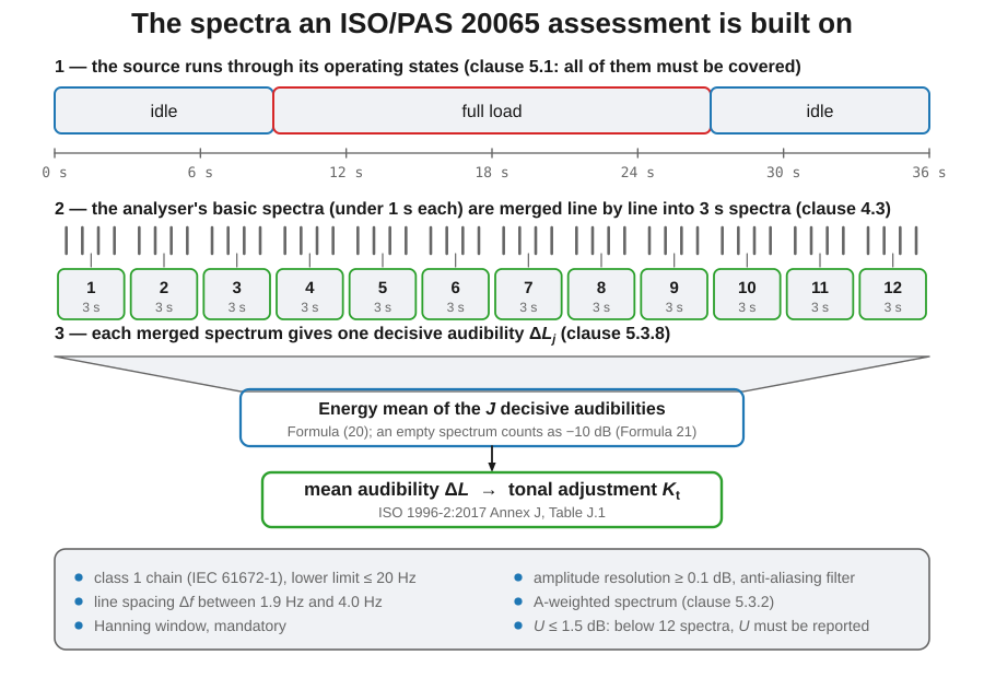
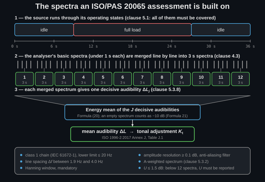
The time structure behind a defensible tonal penalty. The library starts at the third band: it takes merged spectra and returns audibilities, so the first two bands are the caller’s responsibility.

When the method does not apply. A source whose level or tone frequency moves too fast to be represented by a 3 s average cannot be assessed this way at all — start-up transients, strongly speed-varying machinery. Clause 5.1 puts that exclusion in the standard rather than leaving it to judgement.

What the report has to carry (clause 7): date and place; a description of the measurement environment with the source and measurement positions and a sketch of the surroundings; air temperature, air pressure and relative humidity; mean wind speed and direction; the make, model and serial number of every instrument; the line spacing and the frequency range investigated; for every spectrum with a decisive audibility above zero, the tone frequencies and their audibilities; the mean audibility; the extended uncertainty whenever fewer than 12 spectra were averaged; and a plot of the narrow-band levels of the 3 s spectrum with the greatest $\Delta L$. ToneAudibilityResult.report() prints the acoustic half of that list and embeds that plot; the environment and instrument halves arrive through ReportMetadata.

1. The critical band about the tone

Each tone of frequency $f_T$ is evaluated inside a critical band whose width is (Formula 2)

$$\Delta f_c=25.0+75.0{\left(1.0+1.4{\left(\frac{f_T}{1000}\right)}^2\right)}^{0.69}\mathrm{Hz}.$$

With a geometric placement of the corner frequencies about the tone (Formulae 3–5), $\sqrt{f_1{f}_2}=f_T$ and $f_2-f_1=\Delta f_c$, so $f_1=-\Delta f_c/2+\sqrt{\Delta f_c^2+4f_T^2}/2$ and $f_2=f_1+\Delta f_c$.

from phonometry import psychoacoustics

print(round(psychoacoustics.critical_bandwidth_engineering(137.3), 2))   # 101.36 Hz
f1, f2 = psychoacoustics.critical_band_corners(137.3)
print(round(f1, 2), round(f2, 2))                            # 95.67 197.04

2. Audibility of a tone

The mean narrow-band level $L_S$ of the masking noise (Formula 6, an iterative energy average of the lines in the critical band) and the tone level $L_T$ (Formula 8, the energy sum of the tonal lines) are derived from the narrow-band spectrum; mean_narrowband_level and tone_level do this directly (see §4). The critical-band level of the masking noise spreads $L_S$ over the critical bandwidth (Formula 12), the masking index accounts for the ear (Formula 13) and the audibility is their difference (Formula 14):

$$L_G=L_S+10{\log }_{10}\frac{\Delta f_c}{\Delta f},a_v=-2-{\log }_{10}[1+(\frac{f}{502}{)}^{2.5}],\Delta L=L_T-L_G-a_v.$$

A supplied tone is audible when $\Delta L>0$. $\Delta f$ is the line spacing (frequency resolution); the energy sums over $K>1$ lines carry a window correction of $10{\log }_{10}(\Delta f/\Delta f_e)$ (−1.76 dB for the recommended Hanning window, $\Delta f_e=1.5\Delta f$, Formula (8)), while a single-line tone ($K=1$) takes its level unchanged (Formula (7), no bandwidth correction).

from phonometry import psychoacoustics

# ISO/PAS 20065 Annex E, tone at 137.3 Hz (Δf = 2.7 Hz):
#   LS = 49.22 dB (Formula 6), LT = 67.96 dB (Formula 8).
print(round(psychoacoustics.tone_audibility(67.96, 49.22, 137.3, 2.7), 2))   # 5.01 dB
print(round(psychoacoustics.masking_index(137.3), 2))                        # -2.02 dB

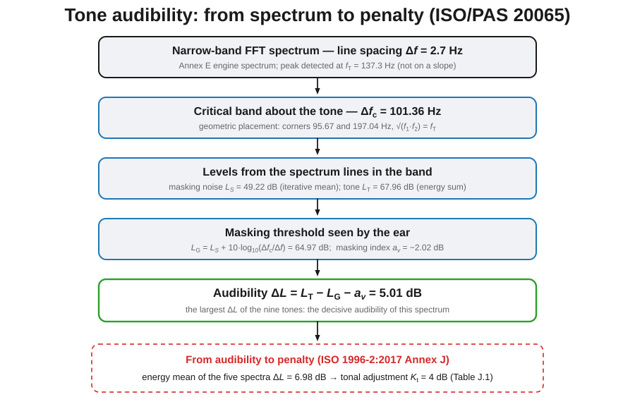
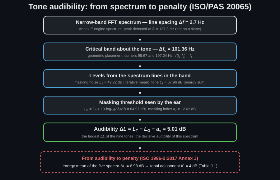
The whole method is one chain from the spectrum to the penalty, and every intermediate quantity above is a stop on it. The diagram walks the Annex E tone through that chain, down to the $K_t$ the mean audibility earns.

3. Decisive and mean audibility

The decisive audibility of one narrow-band spectrum is the largest tone audibility in it (clause 5.3.8). Over $J$ staggered spectra the mean audibility is their energy mean (Formula 20); a spectrum in which no tone is found contributes $\Delta L_j=-10\text{dB}$ (Formula 21). assess_tones is the per-tone entry point: it applies Formulae (2)-(5) and (12)-(14) to each tone it is given and reports the largest, which is the decisive audibility only when no two audible tones share a critical band.

How the decisive band is selected. The method does not scan a fixed set of bands: each detected tone defines its own critical band (§1), the audibility is evaluated tone by tone, and, after Step 3 has merged audible same-band tones into FG groups rated at their most audible member (§5), the decisive audibility is simply the largest $\Delta L$ left standing (Step 4). The “decisive band” is therefore the critical band centred on whichever tone or group wins, and it is free to move from spectrum to spectrum as the source runs through its operating states; the energy mean of Formula 20 then lets the loudest (most audible) spectra dominate the reported value, which is deliberate: a tone that is clearly audible part of the time is not excused by intervals in which it disappears.

from phonometry import psychoacoustics

# Annex E combustion-engine spectrum 1: nine tones (fT, LT, LS), Δf = 2.7 Hz.
fT = [118.4, 137.3, 158.8, 314.9, 433.4, 592.2, 629.8, 643.3, 1582.7]
LT = [64.56, 67.96, 68.63, 68.50, 73.17, 78.31, 75.00, 79.75, 71.07]
LS = [48.91, 49.22, 50.50, 52.85, 58.29, 59.53, 59.71, 61.98, 54.16]
res = psychoacoustics.assess_tones(fT, LT, LS, 2.7)
print(round(res.decisive_audibility, 2), res.decisive_frequency)  # 5.01 137.3

# The five spectra of the Annex E campaign, rated with Step 3 applied
# (Table E.3 decisive values), energy-averaged by Formula 20:
print(round(psychoacoustics.mean_audibility([9.18, 6.04, 7.46, 2.67, 7.17]), 2))  # 6.98 dB

res.plot(view="levels")   # tone levels above their critical-band masking noise

The two numbers in that block are not the same spectrum rated twice by the same rule. The tones at 118.4, 137.3 and 158.8 Hz all fall in one critical band, so clause 5.3.8 Step 3 merges them into an FG group at their combined level $L_T=72.15$ dB, and the standard’s decisive value for spectrum 1 is the 9.18 dB that opens the mean_audibility list — not the 5.01 dB the per-tone call prints, which is the largest of the nine individual audibilities [0.75, 0.89, 1.02, 1.79, 1.93, 3.47, 4.39, 4.57, 5.01]. Those 4.2 dB survive the averaging: the per-tone value in place of 9.18 pulls the campaign mean from 6.98 dB to 5.98 dB, which is $K_t=3$ dB instead of 4 dB in ISO 1996-2 Table J.1. So use analyze_spectrum (§5), which runs the grouping, whenever a decisive audibility is going to be reported, and assess_tones only when the grouping has already been resolved.

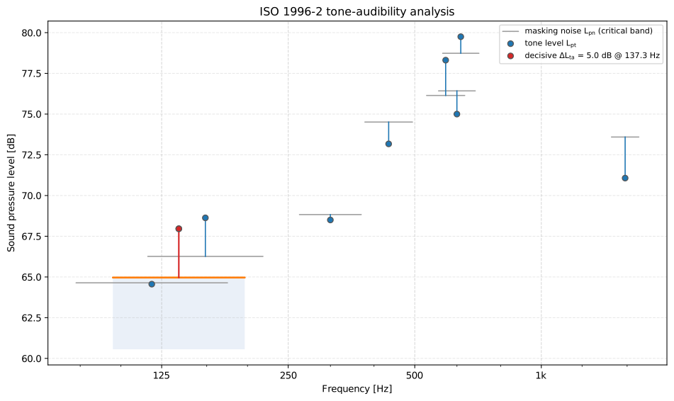
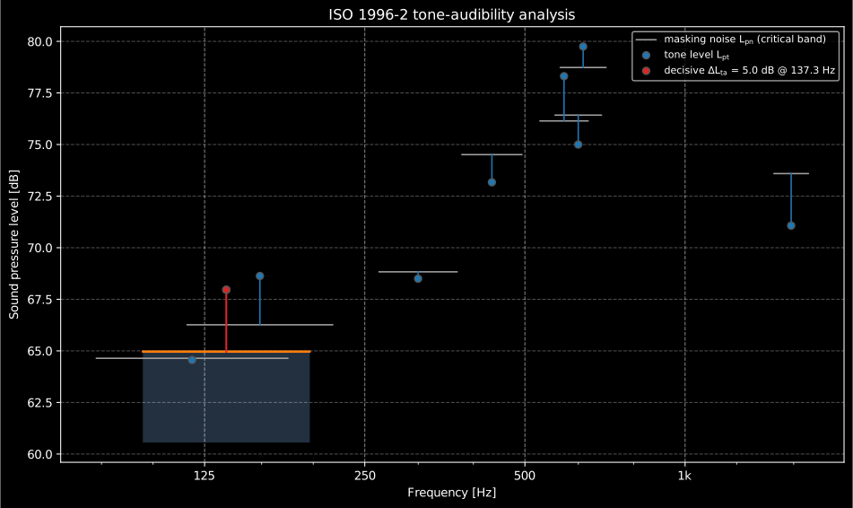
The same assessment reads two ways. The audibility bars at the top of this page answer “how far above the masking threshold is each tone”; the levels view answers “what did the analyser see”, which is the view an assessment report has to defend:

Show the code for this figure

import matplotlib.pyplot as plt
from phonometry import psychoacoustics

# The Annex E combustion-engine spectrum of the snippet above.
fT = [118.4, 137.3, 158.8, 314.9, 433.4, 592.2, 629.8, 643.3, 1582.7]
LT = [64.56, 67.96, 68.63, 68.50, 73.17, 78.31, 75.00, 79.75, 71.07]
LS = [48.91, 49.22, 50.50, 52.85, 58.29, 59.53, 59.71, 61.98, 54.16]
res = psychoacoustics.assess_tones(fT, LT, LS, 2.7)

# One line: the levels view, the same one the .report() fiche embeds.
res.plot(view="levels")
plt.show()

# The default view is the per-tone audibility instead:
res.plot()      # or res.plot(view="audibility")
plt.show()

Reading it left to right: each horizontal segment is the critical-band masking-noise level $L_G$ drawn across the band it applies to, each marker is the tone level $L_T$, and the gap between them, less the masking index, is the audibility. A tone whose marker sits below its segment is masked, and no amount of level justifies a penalty for it.

3.1 Extended uncertainty of the audibility

Clause 5.4 attaches a 90 % bilateral extended uncertainty $U$ to every audibility, and clause 6 makes it mandatory whenever fewer than 12 spectra have been averaged. assess_tones computes it per tone (res.extended_uncertainties), audibility_uncertainty evaluates it straight from the spectrum lines, and mean_audibility_uncertainty propagates it to the energy-averaged audibility of a spectrum set (Annex E: $U=2.80\text{dB}$ for the 137.3 Hz tone against the printed 2,79).

How to read $U$. A 90 % bilateral interval leaves 5 % in each tail, so $\Delta L-U$ is a one-sided 95 % statement: when the whole interval $\Delta L\pm U$ sits above 0 dB the tone is audible with at least 95 % confidence, and when the interval straddles zero the verdict is not statistically secured; the remedy is more spectra, since $U$ shrinks with the number averaged (which is exactly why clause 6 makes reporting it mandatory below 12 spectra). The same logic guards the downstream penalty: ISO 1996-2:2017 Annex J converts the mean audibility into the tonal adjustment $K_t$ in 1 dB steps (Table J.1: $K_t=0$ for $\Delta L\le 0$, up to $K_t=6\text{dB}$ for $\Delta L>12\text{dB}$, or the coarser 0/3/6 dB ladder of its note), so an uncertainty that spans a table boundary propagates straight into a 1–3 dB question mark on the rating level. Quoting $\Delta L\pm U$ alongside $K_t$ shows whether the adjustment is robust or hinges on one borderline spectrum.

The Annex E campaign is exactly that case. Its five 3 s spectra (Table E.4) carry decisive audibilities of 9.18, 6.04, 7.46, 2.67 and 7.17 dB with individual uncertainties of 3.21, 2.95, 2.44, 2.52 and 2.14 dB; the energy mean is 6.98 dB and mean_audibility_uncertainty propagates those into $U=1.38$ dB.

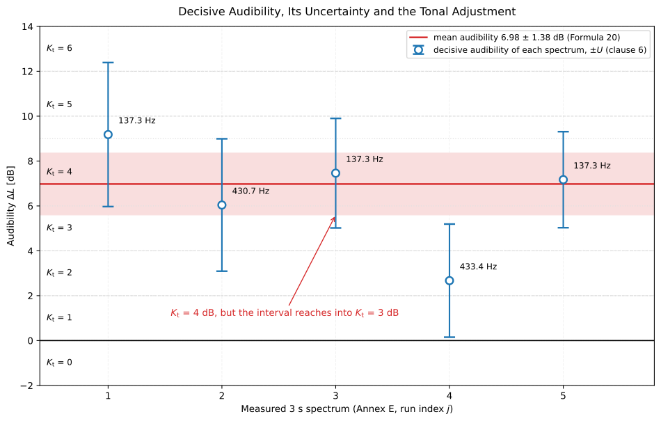
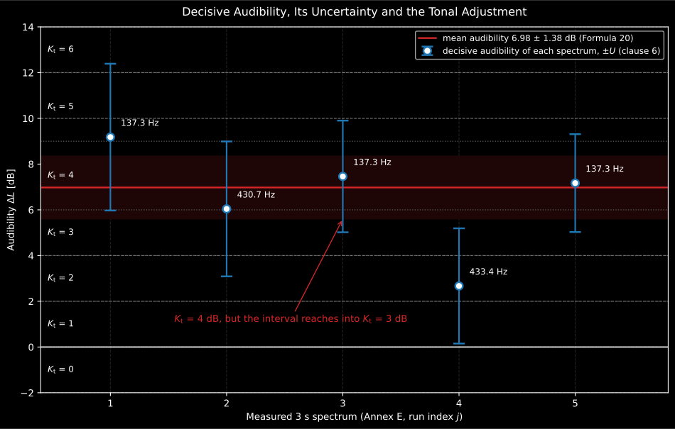
Five spectra, one penalty. The mean audibility earns $K_t=4$ dB, but its uncertainty band reaches below the 6 dB boundary of ISO 1996-2 Table J.1, so $K_t=3$ dB is not excluded — and the remedy is more spectra, not a rounder number.

Show the code for this figure

# `psychoacoustics` is imported by the snippets above.
# ISO/PAS 20065 Annex E Table E.4: one decisive audibility and one extended
# uncertainty per measured 3 s spectrum.
decisive = [9.18, 6.04, 7.46, 2.67, 7.17]
uncertainty = [3.21, 2.95, 2.44, 2.52, 2.14]

mean = psychoacoustics.mean_audibility(decisive)
u = psychoacoustics.mean_audibility_uncertainty(decisive, uncertainty)
print(round(mean, 2), round(u, 2))     # 6.98 1.38 — Kt = 4 dB, Kt(ΔL − U) = 3 dB

4. From the narrow-band spectrum

Given the FFT lines of the critical band about a tone, mean_narrowband_level runs the iterative Formula 6 procedure (energy average, dropping any line more than 6 dB above the running $L_S$, until stable within ±0.005 dB or fewer than five lines remain each side, Annex D) and tone_level sums the tonal lines contiguous with the peak (above both $L_S+6\text{dB}$ and $L_{\text{peak}}-10\text{dB}$). The mean always carries the −1.76 dB Hanning bandwidth correction; the tone level carries it only when the run spans more than one line (Formulae (7)/(8)).

from phonometry import psychoacoustics

# Annex E Table E.1: the 38 lines of the 137.3 Hz critical band (Δf = 2.7 Hz).
freqs = [96.9, 99.6, 102.3, 105.0, 107.7, 110.4, 113.0, 115.7, 118.4, 121.1,
         123.8, 126.5, 129.2, 131.9, 134.6, 137.3, 140.0, 142.7, 145.3, 148.0,
         150.7, 153.4, 156.1, 158.8, 161.5, 164.2, 166.9, 169.6, 172.3, 175.0,
         177.6, 180.3, 183.0, 185.7, 188.4, 191.1, 193.8, 196.5]
levels = [49.40, 50.68, 50.09, 53.37, 44.47, 50.91, 51.41, 59.40, 64.54, 57.57,
          51.02, 50.76, 59.93, 62.94, 58.49, 65.87, 62.66, 50.25, 51.32, 52.30,
          52.58, 53.15, 67.04, 67.27, 57.40, 57.17, 52.56, 51.39, 52.49, 47.68,
          51.26, 49.03, 61.42, 59.52, 48.43, 50.84, 48.20, 55.95]

ls = psychoacoustics.mean_narrowband_level(levels, freqs, 137.3)
lt = psychoacoustics.tone_level(levels, freqs, 137.3, ls)
print(round(ls, 2), round(lt, 2))                         # 49.22 67.96
print(round(psychoacoustics.tone_audibility(lt, ls, 137.3, 2.7), 2))   # 5.01 dB

5. Whole-spectrum detection

analyze_spectrum runs the full front-end over a spectrum (mean narrow-band level per line, peak detection (Clause 5.3.8 Step 1, a tone cannot sit on a slope), tone level, the distinctness test (Clause 5.3.4: bandwidth $\le 26(1+0.001f_T)$ Hz and edge steepness $\ge 24\text{dB}$), and audibility) and returns the distinct, audible tones. It then applies Step 3: audible tones sharing a critical band have their tone levels energy-summed (Formula 17, shared lines counted once, via combined_tone_level) into a combined “FG” entry rated at the most audible member, unless the exactly-two-tones-below-1000-Hz exception of §5.1 keeps them separate. The result’s group_sizes tells individual tones (1) from FG entries ($N\ge 2$), and the decisive audibility (Step 4) is the maximum over all entries.

from phonometry import psychoacoustics

# Annex E Table E.1: the 38 lines of the 137.3 Hz critical band (Δf = 2.7 Hz).
freqs = [96.9, 99.6, 102.3, 105.0, 107.7, 110.4, 113.0, 115.7, 118.4, 121.1,
         123.8, 126.5, 129.2, 131.9, 134.6, 137.3, 140.0, 142.7, 145.3, 148.0,
         150.7, 153.4, 156.1, 158.8, 161.5, 164.2, 166.9, 169.6, 172.3, 175.0,
         177.6, 180.3, 183.0, 185.7, 188.4, 191.1, 193.8, 196.5]
levels = [49.40, 50.68, 50.09, 53.37, 44.47, 50.91, 51.41, 59.40, 64.54, 57.57,
          51.02, 50.76, 59.93, 62.94, 58.49, 65.87, 62.66, 50.25, 51.32, 52.30,
          52.58, 53.15, 67.04, 67.27, 57.40, 57.17, 52.56, 51.39, 52.49, 47.68,
          51.26, 49.03, 61.42, 59.52, 48.43, 50.84, 48.20, 55.95]

# Same Table E.1 spectrum as above.
res = psychoacoustics.analyze_spectrum(levels, freqs, 2.7)
singles = res.group_sizes == 1
print([round(f, 1) for f in res.tone_frequencies[singles]])  # [118.4, 137.3, 158.8]

# Step 3 already combined the three same-band tones into an FG entry:
fg = res.group_sizes > 1
print(int(res.group_sizes[fg][0]), round(float(res.tone_levels[fg][0]), 2))  # 3 72.15

# The same Formula 17 combination, called directly (LS from Table E.2):
lt_fg = psychoacoustics.combined_tone_level(levels, freqs, [118.4, 137.3, 158.8],
                               [48.91, 49.22, 50.50])
print(round(lt_fg, 2))                                # 72.15

res.plot()   # the detected entries, FG groups included, as audibility bars

Reproducing a decisive audibility exactly needs the complete narrow-band spectrum: Table E.1 is truncated to the 137.3 Hz critical band, so the 158.8 Hz tone’s mean narrow-band level is under-estimated from it (the algorithm itself matches the parent standard DIN 45681:2005-03 reference program). The peak detection and FG combination are verified against the Annex E worked example (the three tone frequencies and $L_T=72.15\text{dB}$).

5.1 Two tones below 1000 Hz

When exactly two tones share a critical band and both lie below 1000 Hz, the ear can still tell them apart (so they are rated separately rather than FG-combined) if their frequency difference $|f_{T1}-f_{T2}|$ (Formula 18) exceeds

$$f_D=21\cdot 10^{1.2{|{\log }_{10}(f_T/212)|}^{1.8}}\text{Hz}(\text{Formula 19},88\text{Hz}<f_T<1000\text{Hz})$$

evaluated at the more prominent tone $f_T$ (the larger audibility $\Delta L$). The threshold bottoms out at 21 Hz at $f_T=212\text{Hz}$ and grows on either side. two_tone_separation_frequency gives $f_D$; resolve_tones_separately applies the decision.

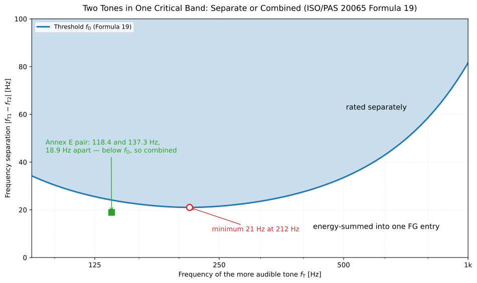
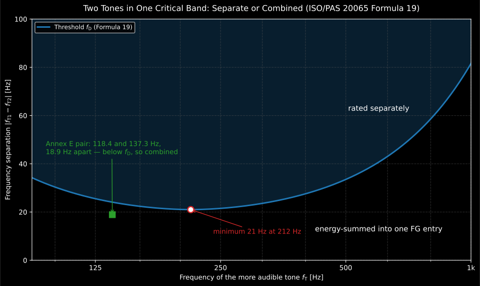
Where the ear stops resolving two tones in one critical band. The threshold is narrowest around 212 Hz and widens steeply above 500 Hz — at 1 kHz two tones must be 82 Hz apart to be rated separately, which is most of the critical band. The Annex E pair sits just below the curve and is therefore combined.

Show the code for this figure

import matplotlib.pyplot as plt
import numpy as np

# `psychoacoustics` is imported by the snippets above.
ft_grid = np.logspace(np.log10(88.0), np.log10(1000.0), 400)
fd = [psychoacoustics.two_tone_separation_frequency(f) for f in ft_grid]

plt.semilogx(ft_grid, fd, label="Threshold fD (Formula 19)")
plt.plot([212.0], [21.0], "o")          # the 21 Hz minimum
plt.plot([137.3], [18.9], "s")          # the Annex E pair, 118.4 and 137.3 Hz
plt.xlabel("Frequency of the more audible tone fT [Hz]")
plt.ylabel("Frequency separation |fT1 - fT2| [Hz]")
plt.legend()
plt.show()

from phonometry import psychoacoustics

psychoacoustics.two_tone_separation_frequency(212.0)             # 21.0 Hz (minimum)
psychoacoustics.resolve_tones_separately(200.0, 260.0, 3.0, 2.0) # True  → rate separately
psychoacoustics.resolve_tones_separately(118.4, 137.3, 4.0, 5.0) # False → combine (Δf < fD)

Note

No ISO/PAS 20065 worked example exercises this branch; the Annex E band groups three tones, so the “exactly two tones” rule never fires there. The formula and decision are implemented clean-room from the text and verified against the DIN 45681:2005-03 Annex J reference program (fD = 21 * 10 ^ (1.2 * Abs(Log(fT / 212) / Log(10)) ^ 1.8)). Reassuringly, evaluated at the Annex E tones the threshold ($\approx 24\text{Hz}$ at 137.3 Hz) keeps them combined, consistent with that example’s FG grouping.

6. Tonal assessment report (.report())

The fiche uses the ISO 1996-2 reporting symbols: the decisive audibility is written $\Delta L_{ta}$ and the tonal adjustment $K$, which are the $\Delta L$ and $K_t$ of the sections above.

ToneAudibilityResult.report(path) renders a one-page PDF fiche laid out like a tonal-assessment report of an environmental-noise laboratory, following the ISO 1996-2:2017 Annex J engineering method: a standard-basis line, an optional metadata header block (source/situation, client, measurement position, instrumentation and date, with the analysis line spacing $\Delta f$ read from the result), a full-width table of the key quantities for every detected tone (tone frequency $f_T$, entry type, tone level $L_{pt}$, critical-band masking-noise level $L_{pn}$, critical bandwidth $\Delta f_c$ and the audibility $\Delta L_{ta}$) above the level-versus-frequency analysis plot with the tones and their critical-band masking noise marked, the boxed decisive audibility $\Delta L_{ta}$ together with the derived tonal adjustment $K$ (Table J.1), an optional PASS/FAIL verdict row and a prominence note, and a footer with the fixed disclaimer.

It uses the same ReportMetadata container and rendering engine as the ISO 532-1 loudness fiche; a supplied requirement is read as the maximum acceptable decisive audibility $\Delta L_{ta}$ in dB (a quieter tone passes). Rendering needs reportlab and, for the figure the fiche embeds, matplotlib (pip install "phonometry[report,plot]"); only engine="reportlab" is supported. The fiche renders in English by default; pass language="es" for a Spanish fiche (translated fixed strings and a comma decimal separator), e.g. res.report("tone_fiche_es.pdf", language="es").

from phonometry import psychoacoustics, ReportMetadata

# The Annex E combustion-engine spectrum from §4/§5 (analyze_spectrum).
res = psychoacoustics.analyze_spectrum(levels, freqs, 2.7)
res.report(
    "tone_fiche.pdf",
    metadata=ReportMetadata(
        specimen="Combustion engine, steady operation",
        measurement_standard="ISO 1996-2",
        laboratory="Phonometry Reference Laboratory",
        requirement=6.0,             # maximum acceptable ΔL_ta (dB)
    ),
)                                    # decisive ΔL_ta (dB) and K (dB, Table J.1)

The example fiche is regenerated with make reports and kept rendered in the repository; click the preview to open the PDF.

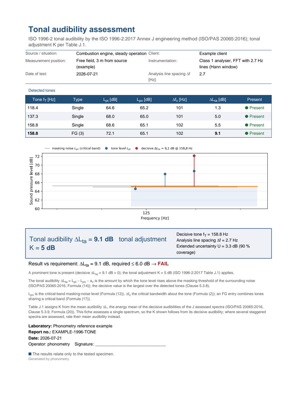
One-page tonal-assessment fiche: a metadata header, a per-tone table of the tone level Lpt, the critical-band masking-noise level Lpn, the critical bandwidth and the audibility, the level-versus-frequency analysis plot with the tones and their masking noise marked, the boxed decisive ΔL_ta = 9.1 dB with the tonal adjustment K = 5 dB (ISO 1996-2:2017 Table J.1) and a FAIL verdict against a 6 dB audibility limit.

Download the report (PDF)

Tonal audibility fiche (ToneAudibilityResult.report), decisive ΔL_ta in dB with the tonal adjustment K.

What this guide covers

• Covered

  The ISO/PAS 20065:2016 engineering method in full: the clause 4.2 analyser requirements and the clause 4.3 merging of basic spectra that the input rests on, with the clause 5.1 acceptance conditions and the clause 7 reporting list; the critical bandwidth $\Delta f_c$ and corner frequencies (Formulae 2 to 5), the mean narrow-band level $L_S$ and tone level $L_T$ (Formulae 6 and 8, Annex D), the critical-band masking level $L_G$, the masking index $a_v$ and the audibility $\Delta L$ (Formulae 12 to 14), peak detection and the distinctness test (clauses 5.3.8 and 5.3.4), the multi-tone FG combination (Formula 17) and the two-tones-below-1000-Hz exception (Formulae 18/19), the decisive and energy-mean audibility (Formula 20) and the clause 5.4/6 extended uncertainty $U$, all through psychoacoustics.analyze_spectrum and assess_tones. ISO 1996-2:2017 Annex J is covered as far as it maps the mean audibility to the tonal adjustment $K_t$ (Table J.1).

• Not covered

  The distinctness edge-steepness test follows the DIN 45681:2005-03 reading (its executable reference program), not the asymmetric formulas printed in the ISO/PAS 20065 text, which contradict it, recorded in the errata registry. Building the narrow-band FFT spectrum itself from a raw time-domain recording is not part of this module: every function here takes an already-computed spectrum (levels and frequencies), and §0 states what that spectrum has to be — including the clause 5.3.2 A-weighting, which the caller applies because the module is weighting agnostic.

See also

• Environmental noise measurement: the ISO 1996-1 rating level this audibility feeds, and the simpler ISO 1996-2 Annex C route for a single spectrum.
• Tone prominence: TNR and PR: the ECMA-418-1 prominence question asked of product noise, with the table that picks between the library’s four tonality metrics.
• Wind turbine noise: the IEC 61400-11 per-bin audibility, the same formula applied to a bin-by-bin wind-speed campaign.
• Theory: the neighbouring family of tone metrics, TNR and PR, derived from the same critical-band picture.
• API reference: psychoacoustics.quality.tone_audibility.

References

• Deutsches Institut für Normung. (2005). Akustik — Bestimmung der Tonhaltigkeit von Geräuschen und Ermittlung eines Tonzuschlages für die Beurteilung von Geräuschimmissionen (DIN 45681:2005-03). The parent standard the −1.76 dB Hanning bandwidth correction, the iterative masking-level procedure and the detection/combination logic are confirmed against (its Annex J reference program).
• International Organization for Standardization. (2016). Acoustics — Objective method for assessing the audibility of tones in noise — Engineering method (ISO/PAS 20065:2016). The implemented engineering method: every formula on this page follows the 2016 PAS edition. The critical bandwidth Δfc (Formula 2) and its corner frequencies (Formulae 3–5), the critical-band level LG (Formula 12), the masking index av (Formula 13), the audibility ΔL = LT − LG − av (Formula 14) and the energy-mean mean audibility (Formula 20); the mean narrow-band level LS (Formula 6, iterative Annex D) and tone level LT (Formula 8) come from the critical-band spectrum, and analyze_spectrum adds peak detection (Clause 5.3.8) with the distinctness criteria (Clause 5.3.4), the multi-tone FG combination (Formula 17) and the separate evaluation of two tones below 1000 Hz (Formulae 18/19). Conformance is anchored on the Annex E combustion-engine worked example (Tables E.1/E.2/E.3). Withdrawn, superseded by ISO/TS 20065:2022 (https://www.iso.org/standard/81518.html).
• International Organization for Standardization. (2017). Acoustics — Description, measurement and assessment of environmental noise — Part 2: Determination of sound pressure levels (ISO 1996-2:2017). The environmental-noise standard this method serves: its Annex J adopts the engineering method and maps the mean audibility to the tonal adjustment Kt (Table J.1) discussed in §3.1.