Advanced Loudness (ISO 532-2/-3, ECMA-418-2)

The Zwicker method of ISO 532-1 is the reference route to loudness in sones and lives in Loudness, together with the ISO 226 equal-loudness contours. This page covers the newer model families phonometry ships beside it: the Moore-Glasberg loudness of ISO 532-2/532-3 and the Sottek Hearing Model loudness of ECMA-418-2:2025, whose shared auditory front-end also powers the tonality and roughness metrics of Sound Quality Metrics.

The page opens with the choice: which model fits which measurement, and why the sone values of the four methods agree at the 1 kHz / 40 dB anchor yet are not interchangeable digit for digit. Each model then gets its own section with a worked example, its figure and its parameter table.

Choosing a loudness model

Model	Standard	Stationary / time-varying	Output	When to use
Zwicker	ISO 532-1:2017	both	sone	Reference method; one-third-octave input; fast and widely cited
Moore-Glasberg	ISO 532-2:2017	stationary	sone	roex excitation pattern; better for tones and explicit binaural summation
Moore-Glasberg-Schlittenlacher	ISO 532-3:2023	time-varying	sone (STL/LTL)	Time-varying loudness with short-/long-term traces and the peak $N_{\text{max}}$
Sottek (Hearing Model)	ECMA-418-2:2025	time-varying	sone_HMS	Shares one auditory front-end with the ECMA tonality and roughness metrics

All four methods are anchored so a 1 kHz tone at 40 dB SPL is ≈ 1 sone; the values are not interchangeable digit-for-digit because the models differ in their auditory filters and their loudness summation.

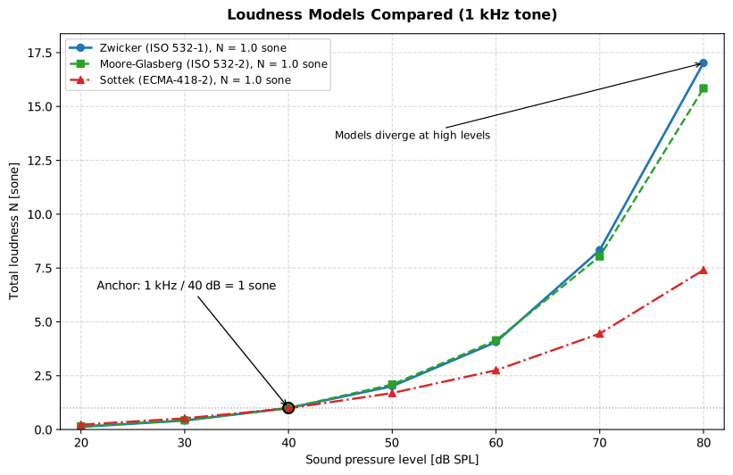
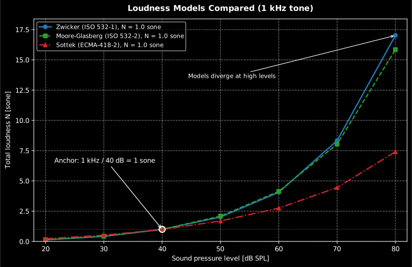
The three models pass through approximately 1 sone at the 40 dB anchor (the Sottek front-end returns 0.9845 sone_HMS there) and diverge with level: Zwicker doubles the sone value every +10 phon, while the Sottek model grows more slowly (about 1.65× per 10 dB), an intrinsic difference between the auditory summations, not a calibration error.

Show the code for this figure

import matplotlib.pyplot as plt
import numpy as np
from phonometry import psychoacoustics

# 1 kHz tone, 20..80 dB SPL: all three models pass close to 1 sone at 40 dB
fs = 48000
t = np.arange(fs) / fs
levels = np.arange(20.0, 81.0, 10.0)
zw, mg, ec = [], [], []
for spl in levels:
    x = np.sqrt(2) * 2e-5 * 10 ** (spl / 20) * np.sin(2 * np.pi * 1000 * t)
    zw.append(psychoacoustics.loudness_zwicker(x, fs, stationary=True).loudness)
    mg.append(
        psychoacoustics.loudness_moore_glasberg_from_spectrum([(1000.0, float(spl))]).loudness
    )
    ec.append(psychoacoustics.loudness_ecma(x, fs).loudness)

fig, ax = plt.subplots()
ax.plot(levels, zw, "o-", label="Zwicker (ISO 532-1)")
ax.plot(levels, mg, "s--", label="Moore-Glasberg (ISO 532-2)")
ax.plot(levels, ec, "^-.", label="Sottek (ECMA-418-2)")
ax.plot(40.0, 1.0, "o", color="k", markerfacecolor="none", markersize=10)   # the shared anchor
ax.set(xlabel="Sound pressure level [dB SPL]", ylabel="Total loudness N [sone]")
ax.legend()
plt.show()

The ERB_N scale and the Cam axis

Every model on this page except Zwicker’s is written on the ERB_N number axis, so it is worth having the scale itself in hand. The cochlea behaves as a bank of overlapping band-pass auditory filters; the width of the one centred on a given frequency is summarised by its equivalent rectangular bandwidth, the bandwidth of the rectangular filter that would pass the same power with the same peak response. Fitting notched-noise data for young listeners at moderate levels, Glasberg and Moore (1990) make it a straight line in frequency (Moore, An Introduction to the Psychology of Hearing 6e, p. 76):

$${\mathrm{ERB}}_N=24.7(4.37F+1)\text{Hz},F\text{ in kHz}.$$

Integrating $df/{\mathrm{ERB}}_N(f)$ turns that into a frequency scale on which one step is one auditory-filter width. The scale is the ERB_N number and its unit is the Cam, after Cambridge:

$${\mathrm{ERB}}_N\text{number}=21.4{\log }_{10}(4.37F+1)\text{Cam}.$$

from phonometry import psychoacoustics

cam = psychoacoustics.cam_from_frequency(1000.0)
print(round(psychoacoustics.erb_bandwidth(1000.0), 1))       # 132.4 Hz
print(round(cam, 2))                                         # 15.59 Cam
print(round(psychoacoustics.frequency_from_cam(cam), 1))     # 1000.0 Hz

The library states the same fit with one more significant digit, ${\mathrm{ERB}}_N=24.673(0.004368f+1)$ and $21.366{\log }_{10}(0.004368f+1)$, the precision the ISO 532-2 implementation uses; the two forms agree to better than 0.2 % over the audible range, and the extra digits are what make frequency_from_cam an exact inverse. These are not private helpers of the loudness model: loudness_moore_glasberg calls the same three functions, so a MooreGlasbergLoudness.erb_number grid and a Cam axis you build yourself cannot drift apart.

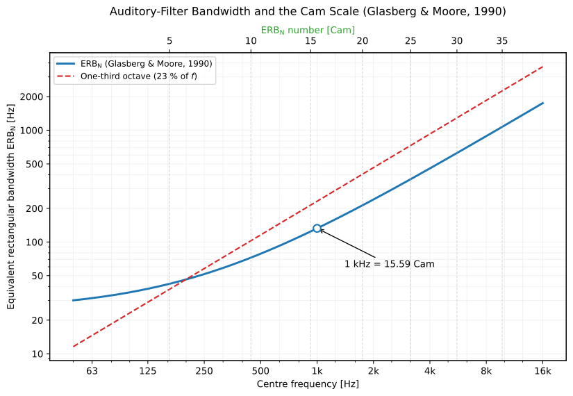
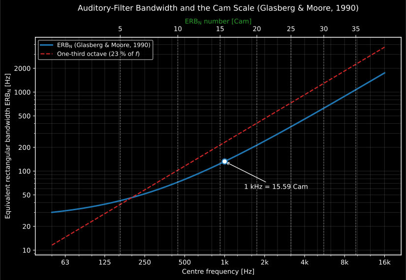
The ear’s filter is not a constant fraction of frequency. Below about 500 Hz it is markedly narrower than a one-third octave, which is why the “old” critical-band function, flat at low frequency, fits the direct measurements so poorly there; above that it is wider. The top axis counts the same curve in Cams, so equal steps along it are equal numbers of auditory filters.

Show the code for this figure

import matplotlib.pyplot as plt
import numpy as np
from phonometry import psychoacoustics

f = np.geomspace(50.0, 16000.0, 400)
erb = psychoacoustics.erb_bandwidth(f)
third_octave = f * (2 ** (1 / 6) - 2 ** (-1 / 6))     # 23 % of f, for scale

fig, ax = plt.subplots()
ax.loglog(f, erb, label="ERB$_N$ (Glasberg & Moore, 1990)")
ax.loglog(f, third_octave, "--", label="One-third octave (23 % of f)")
ax.set(xlabel="Centre frequency [Hz]",
       ylabel="Equivalent rectangular bandwidth ERB$_N$ [Hz]")
ax.legend()

# The Cam axis on top: tick where whole ERB_N numbers fall.
cam_ticks = np.arange(5.0, 40.0, 5.0)
ax2 = ax.twiny()
ax2.set_xscale("log")
ax2.set_xlim(ax.get_xlim())
ax2.set_xticks(psychoacoustics.frequency_from_cam(cam_ticks))
ax2.set_xticklabels([f"{c:.0f}" for c in cam_ticks])
ax2.set_xlabel("ERB$_N$ number [Cam]")
plt.show()

erb_bandwidth(), cam_from_frequency(), frequency_from_cam() parameters

Parameter	Type	Units	Range / default	Notes
frequency	float or array	Hz	≥ 0	erb_bandwidth, cam_from_frequency
cam	float or array	Cam	≥ 0	frequency_from_cam

Each returns a float for a scalar input and an array otherwise. The three constants are exported as ERB_C1, ERB_C2 and CAM_C.

Moore-Glasberg loudness (ISO 532-2)

Which recording maps to which arguments

field and presentation are not preferences: they are descriptions of how the sound reached the listener, and getting them wrong costs more than any difference between the models on this page. ISO 532-2 clause 7.2 lists the listening situations and the transfer function each needs, and clause 8.1 fixes what the two ears do with the result.

How the sound was captured	field=	Why
One microphone at the centre of the position the absent listener’s head would occupy, one frontal source	'free'	Table 1 column 2, the free-field transfer to the tympanic membrane
The same microphone in a reverberant room or in situ	'diffuse'	Table 1 column 3, the diffuse-field transfer; also the right choice for diffuse-field earphones
A probe microphone within 10 mm of the eardrum (5 mm when there are strong components above 3 kHz)	'eardrum'	Clause 7.2.4: the spectrum is already at the membrane, so no transfer function is applied
A head-and-torso simulator	'eardrum', but only if the simulator is an accurate acoustical model of an average adult	Clause 7.2.5; otherwise it needs its own correction file, which this API cannot express — equalize the recording to the free or diffuse field first and use the matching option

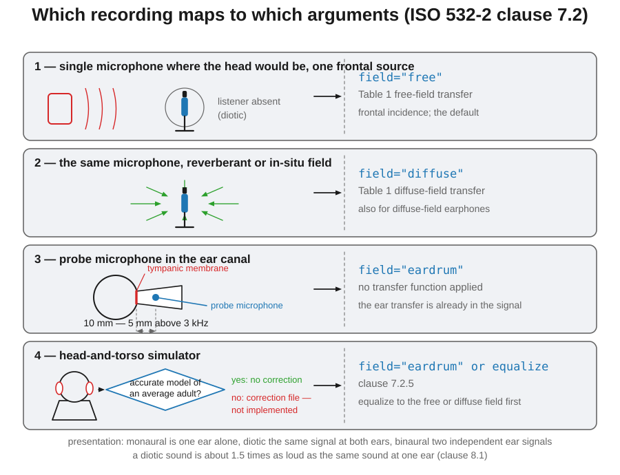
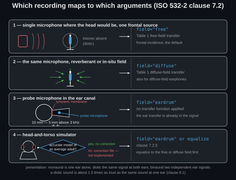
The four situations of clause 7.2, with the geometry that decides them. The distances in scene 3 are the standard’s own: 10 mm from the tympanic membrane, 5 mm when the sound has strong components above 3 kHz.

The failure mode is silent and large. Applying a free-field transfer to a signal that already contains the ear-canal resonance double-counts a gain of about 15 dB near 3 kHz: a 3 kHz tone at 70 dB reads 13.8 sone (78.0 phon) with field="free" and 5.0 sone (62.7 phon) with field="eardrum", and nothing in the result says which of the two was appropriate. In the other direction, a free-field recording analysed as 'eardrum' under-reads by the same amount.

presentation is the other factor of two. monaural computes one ear with the other silent, diotic presents the identical signal to both ears — which is what a single free-field microphone recording represents, since both ears hear the same field — and binaural combines two independent ear signals through the standard’s inhibition stage. The definitional 1 kHz tone at 40 dB is 1.000 sone diotically and 0.667 sone monaurally, the 1.5 ratio clause 8.1 states, and the inhibition is why two ears give about one and a half times one ear rather than exactly twice. For a single-spectrum input binaural and diotic coincide, so the distinction only bites for the two-channel input of loudness_moore_glasberg_time. Note also that loudness_ecma() offers only 'free' and 'diffuse', so eardrum-referenced material has to be corrected before it reaches the ECMA-418-2 model.

Where Zwicker uses fixed critical bands on the Bark scale, Moore-Glasberg builds an excitation pattern with level-dependent rounded-exponential (roex) auditory filters on the ERB-number (“Cam”) scale, then applies a compressive excitation → specific-loudness transform with $C=0.0617\text{sone/Cam}$ (ISO 532-2:2017, Formula 7) and a binaural-inhibition stage. It reproduces the tone and broadband cases of Annex B to a percent or two and, unlike ISO 532-1, models binaural summation explicitly.

import numpy as np
from phonometry import psychoacoustics

# The definitional anchor: one 1 kHz sinusoidal component at 40 dB SPL,
# free field, binaural -> 1 sone / 40 phon by construction of the sone.
res = psychoacoustics.loudness_moore_glasberg_from_spectrum([(1000.0, 40.0)], field="free")
print(f"N = {res.loudness:.3f} sone  ({res.loudness_level:.1f} phon)")   # 1.000 sone (40.0 phon)

# From a calibrated recording: the narrowband (FFT) line spectrum is formed
# (power-preserving normalization) and fed to the exact sinusoidal-component
# method (ISO 532-2 clauses 5.2/5.4).
fs = 48000
x = np.sqrt(2) * 2e-5 * 10 ** (40 / 20) * np.sin(2 * np.pi * 1000 * np.arange(fs) / fs)
res = psychoacoustics.loudness_moore_glasberg(x, fs, field="free", presentation="binaural")

res.plot()   # specific loudness N'(i) over the ERB-number (Cam) scale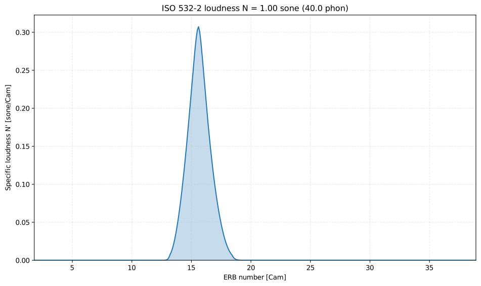

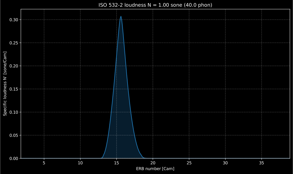
The ISO 532-2 pattern of the definitional 1 sone anchor. The peak is not a spectral line but the excitation the roex filters produce around the tone, so its width is the auditory filter, not the analysis resolution.

Show the code for this figure

import matplotlib.pyplot as plt
import numpy as np
from phonometry import psychoacoustics

# From a calibrated recording: the narrowband (FFT) line spectrum is formed
# (power-preserving normalization) and fed to the exact sinusoidal-component
# method (ISO 532-2 clauses 5.2/5.4).
fs = 48000
x = np.sqrt(2) * 2e-5 * 10 ** (40 / 20) * np.sin(2 * np.pi * 1000 * np.arange(fs) / fs)
res = psychoacoustics.loudness_moore_glasberg(x, fs, field="free", presentation="binaural")

# One line — the specific-loudness pattern N'(i) straight from the result:
res.plot()
plt.show()

# Or draw it by hand from the ERB-number grid the result already carries:
fig, ax = plt.subplots()
ax.fill_between(res.erb_number, res.specific, alpha=0.3)
ax.plot(res.erb_number, res.specific)
ax.set_xlabel("ERB number [Cam]")
ax.set_ylabel("Specific loudness N' [sone/Cam]")
plt.show()

From a one-third-octave spectrum (clause 5.5)

The exact method wants sinusoidal components, but clause 5.5 defines the input a meter actually delivers: the levels of the 29 adjacent one-third-octave bands from 25 Hz to 16 kHz on the IEC 61260-1:2014 nominal centres. Each band is assumed flat and expanded internally into an equivalent set of components before the exact method runs. Two constraints are worth stating plainly: exactly 29 values, and a fixed grid — a meter that logs 20 Hz to 20 kHz has to be trimmed to it, and one that stops at 8 kHz cannot be used at all.

# `psychoacoustics` is imported by the snippets above.
# A ventilation spectrum as a sound level meter logs it: 29 one-third-octave
# bands, 25 Hz to 16 kHz, in dB SPL.
band_levels = [42.0, 45.0, 48.0, 51.0, 54.0, 56.0, 57.0, 57.0, 56.0, 55.0,
               54.0, 53.0, 52.0, 51.0, 50.0, 49.0, 48.0, 47.0, 46.0, 45.0,
               43.0, 41.0, 39.0, 37.0, 34.0, 31.0, 28.0, 25.0, 22.0]

n_mg = psychoacoustics.loudness_moore_glasberg_from_third_octave(
    band_levels, field="diffuse")
print(f"{n_mg.loudness:.1f} sone  ({n_mg.loudness_level:.1f} phon)")  # 17.4 sone (81.3 phon)

# The same measurement through ISO 532-1, which stops one band earlier:
n_zw = psychoacoustics.loudness_zwicker_from_spectrum(
    band_levels[:28], field="diffuse")
print(f"{n_zw.loudness:.1f} sone  ({n_zw.loudness_level:.1f} phon)")  # 13.8 sone (77.9 phon)

The two standards do not even agree on where the spectrum ends: ISO 532-2 takes 29 bands to 16 kHz, ISO 532-1 takes 28 to 12.5 kHz, which is why the slice is needed. The rest of the gap is the models: roex excitation and explicit binaural summation against the ISO 532-1 core loudness. Use field="diffuse" for a room measurement made with a free-field-corrected meter — the field argument is where band-level users most often go wrong.

loudness_moore_glasberg() and its _from_spectrum / _from_third_octave variants

The three entry points differ only in how the spectrum is supplied and share field and presentation.

Parameter	Applies to	Type	Units	Range / default	Notes
x	loudness_moore_glasberg	1D array	Pa	non-empty	Calibrated pressure signal
fs	loudness_moore_glasberg	int	Hz	> 0
components	_from_spectrum	list of (f, L)	Hz, dB SPL	—	Discrete sinusoidal components
band_levels	_from_third_octave	29-vector	dB SPL	25 Hz .. 16 kHz	IEC 61260-1 nominal centres; exactly 29
field	all three	str	—	'free' (default) / 'diffuse' / 'eardrum'	Outer-ear transfer (clause 7.2)
presentation	all three	str	—	'binaural' (default) / 'diotic' / 'monaural'	Binaural summation (clause 8.1)

Returns a MooreGlasbergLoudness: loudness ($N$, sone), loudness_level (phon), specific ($N^{\prime }(i)$, 372 bins of 0.1 Cam), erb_number, centre_frequencies, field, presentation.

Time-varying loudness (ISO 532-3)

ISO 532-3 wraps the same excitation / specific-loudness model in a running multi-resolution spectral analysis (six parallel FFTs, updated every 1 ms) and two cascaded temporal integrators: the fast short-term loudness $S^{\prime }(t)$ and the slower long-term loudness $S^{\prime \prime }(t)$. The peak long-term loudness $N_{\text{max}}$ predicts the loudness of sounds up to about 5 s.

import numpy as np
from phonometry import psychoacoustics

fs = 32000
t = np.arange(int(1.3 * fs)) / fs
x = np.sqrt(2) * 2e-5 * 10 ** (40 / 20) * np.sin(2 * np.pi * 1000 * t)

res = psychoacoustics.loudness_moore_glasberg_time(x, fs, field="free")
print(f"N_max = {res.n_max:.3f} sone  ({res.loudness_level_max:.0f} phon)")   # 1.000 sone (40 phon)
print(f"long-term loudness exceeded 5% of the time: {res.percentiles[5.0]:.3f} sone")   # 0.999 sone

res.plot()   # short-term S'(t) and long-term S''(t) loudness vs time

The short-term loudness rises within a few tens of milliseconds and falls back slowly, mimicking the ear’s fast onset sensitivity and its slower recovery; the long-term loudness integrates that trace again with a much longer time constant, so it barely reacts to a single syllable and instead tracks the overall level of an event. The peak of that slow trace, $N_{\text{max}}$, is the standard’s predictor of the loudness of a short sound, and its validity stops at roughly 5 s because beyond that a listener stops judging the sound as one event. That is also why the percentiles sit beside it: for a sound that fluctuates without a clear event structure, a percentile of the long-term loudness (typically the 5 % value) is the stable statistic, where $N_{\text{max}}$ would be set by the single worst moment.

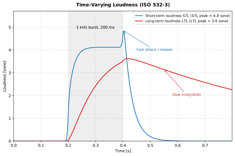
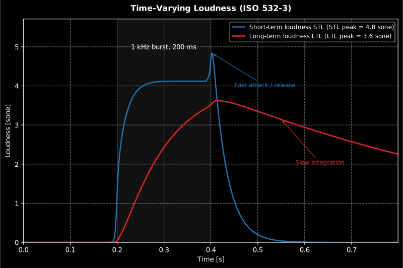
A 200 ms 1 kHz burst at 60 dB SPL: the short-term loudness reaches 4.8 sone within a few tens of milliseconds and releases quickly, while the long-term loudness integrates to 3.6 sone and decays slowly after the burst ends — the pair of time constants ISO 532-3 clauses 7.8/7.9 define.

Show the code for this figure

import matplotlib.pyplot as plt
import numpy as np
from phonometry import psychoacoustics

# The figure is a burst, not a steady tone: 1 kHz at 60 dB SPL, gated on
# between 200 and 400 ms of an 0.8 s record.
fs = 48000
t = np.arange(int(0.8 * fs)) / fs
sig = np.zeros_like(t)
on = (t >= 0.2) & (t < 0.4)
sig[on] = np.sqrt(2) * 2e-5 * 10 ** (60 / 20) * np.sin(2 * np.pi * 1000 * t[on])
burst = psychoacoustics.loudness_moore_glasberg_time(sig, fs)
print(round(float(burst.short_term_loudness.max()), 1),
      round(float(burst.long_term_loudness.max()), 1))   # 4.8  3.6

# The result carries both traces on a 1 ms time axis:
burst.plot()
plt.show()

loudness_moore_glasberg_time() parameters

Parameter	Type	Units	Range / default	Notes
signal	1D or (n, 2) array	Pa	non-empty	Mono = diotic; two columns = left/right ears
fs	int	Hz	> 0
field	str	—	'free' (default) / 'diffuse' / 'eardrum'	Outer-ear transfer
presentation	str	—	'binaural' (default) / 'diotic' / 'monaural'	Binaural summation
percentiles	sequence	percent	default (1, 5, 10, 50, 90, 95)	Exceeded long-term loudness levels

Returns a MooreGlasbergTimeVaryingLoudness: time (1 ms grid), short_term_loudness / long_term_loudness (sone), their _level in phon, n_max, loudness_level_max, a percentiles dict, field, presentation.

Sottek Hearing Model loudness (ECMA-418-2)

ECMA-418-2:2025 specifies a single auditory front-end (outer/middle-ear filtering, a 53-band gammatone-like filter bank on the Bark_HMS scale with $z=0.5..26.5$, half-wave rectification, block RMS and a compressive nonlinearity, Formula 23) that is shared by its loudness, tonality and roughness metrics. The loudness $N$ is reported in sone_HMS, and the same 1 kHz/40 dB anchor calibrates the front-end. The clean-room implementation returns 0.9845 sone_HMS for that anchor rather than exactly 1: the 1.55 % residual comes from the mandated Clause 6.2.3 band averaging across the block-size-boundary bands excited by the tone’s lower flank, near 800 to 900 Hz — without any band averaging the chain reads 0.955, with averaging restricted to same-block-size neighbours 0.996, and with the full cross-group recomputation the standard requires 0.9845. The calibration constant $c_N$ is kept at its verbatim tabulated value rather than retuned, which is why the deviation is visible at all; the psychoacoustics.loudness.ecma API reference carries the full account.

import numpy as np
from phonometry import psychoacoustics

fs = 48000
t = np.arange(int(1.2 * fs)) / fs
x = np.sqrt(2) * 2e-5 * 10 ** (40 / 20) * np.sin(2 * np.pi * 1000 * t)

res = psychoacoustics.loudness_ecma(x, fs, field="free")
print(f"N = {res.loudness:.4f} sone_HMS")   # 0.9845 sone_HMS
print(res.specific_loudness.shape)          # (53,) average specific loudness N'(z)

res.plot()   # average specific loudness N'(z) + time-dependent N(l) at 187.5 Hz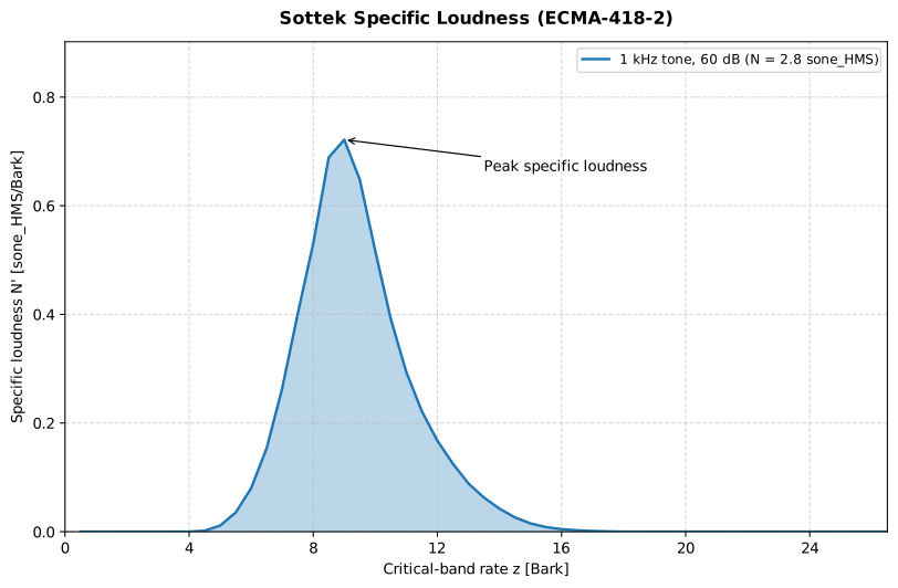

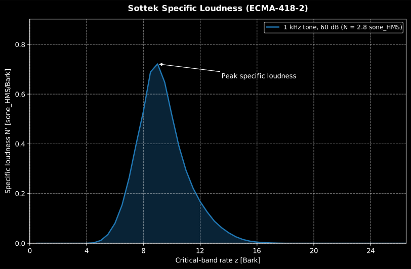
The 1 kHz tone at 60 dB SPL, N = 2.8 sone_HMS — a louder tone than the 40 dB anchor of the snippet above, which gives 0.98 sone_HMS. The loudness is the area under $N^{\prime }(z)$, so a broadband sound spreading a low pattern over many bands can outweigh this single peak.

Show the code for this figure

import matplotlib.pyplot as plt
import numpy as np
from phonometry import psychoacoustics

# The figure is the 60 dB tone, not the 40 dB anchor of the snippet above.
fs = 48000
t = np.arange(int(1.2 * fs)) / fs
x = np.sqrt(2) * 2e-5 * 10 ** (60 / 20) * np.sin(2 * np.pi * 1000 * t)
res = psychoacoustics.loudness_ecma(x, fs, field="free")
print(f"N = {res.loudness:.1f} sone_HMS")   # 2.8 sone_HMS

# The result carries the average specific loudness over the 53 Bark_HMS bands:
res.plot()
plt.show()

# Or draw N'(z) by hand against the critical-band-rate scale:
fig, ax = plt.subplots()
ax.fill_between(res.bark, res.specific_loudness, alpha=0.3)
ax.plot(res.bark, res.specific_loudness)
ax.set_xlabel("Critical-band rate z [Bark_HMS]")
ax.set_ylabel("Specific loudness N' [sone_HMS/Bark_HMS]")
plt.show()

loudness_ecma() parameters

Parameter	Type	Units	Range / default	Notes
signal_in	1D array	Pa	non-empty	Calibrated pressure signal
fs	float	Hz	> 0	Resampled to 48 kHz internally if needed (Clause 5.1.1)
field	str	—	'free' (default) / 'diffuse'	Outer/middle-ear filter (Clause 5.1.3)

Returns an EcmaLoudness: loudness ($N$, sone_HMS), specific_loudness ($N^{\prime }(z)$, 53 bands), bark, centre_frequencies, time, loudness_vs_time ($N(l)$ at 187.5 Hz), field.

What this guide covers

• Covered

  The Glasberg and Moore (1990) ERB_N bandwidth and Cam scale of Moore 6e pp. 76-77, via erb_bandwidth(), cam_from_frequency() and frequency_from_cam(). ISO 532-2:2017 (Moore-Glasberg): the roex excitation pattern of clause 7 and the binaural inhibition of clause 8, via loudness_moore_glasberg() and its _from_spectrum/_from_third_octave variants. ISO 532-3:2023 (Moore-Glasberg-Schlittenlacher): the short-term loudness of clause 7.8, the long-term loudness of clause 7.9 and its peak $N_{\text{max}}$, via loudness_moore_glasberg_time(). ECMA-418-2:2025 (Sottek Hearing Model): the loudness assembly of Clause 8, via loudness_ecma().

• Not covered

  ECMA-418-2’s binaural combination (Formula 118, Clause 8.1.5) is not implemented: loudness_ecma() is monaural, so analyse each ear channel separately. ISO 532-3 Clause 5 prescribes resampling the input to 32 kHz before the running FFT analysis. This implementation processes at the native sampling rate instead, a documented deviation that stays inside the standard’s expanded uncertainty. Resample to 32 kHz first if strict clause-by-clause conformance matters.

See also

• Loudness: the Zwicker reference method (ISO 532-1), its accredited fiche and the ISO 226 equal-loudness contours.
• Sound Quality Metrics: the tonality, roughness and fluctuation strength built on the same ECMA-418-2 front-end.
• Theory: the equations behind the loudness models.
• API reference: psychoacoustics.loudness.moore_glasberg, psychoacoustics.loudness.moore_glasberg_time and psychoacoustics.loudness.ecma.
• Theory: Advanced loudness models and sound quality: what the Moore-Glasberg and Sottek models change relative to Zwicker, and why the three disagree where they do.

Quick answers

Which loudness model should I choose: Zwicker, Moore-Glasberg or Sottek?

The Zwicker method (ISO 532-1:2017) is the reference: stationary and time-varying, one-third-octave input, fast and widely cited. Moore-Glasberg (ISO 532-2:2017) is stationary, builds roex excitation patterns and models binaural summation explicitly; ISO 532-3:2023 adds time-varying short- and long-term loudness with the peak $N_{\text{max}}$. The Sottek model (ECMA-418-2:2025) reports sone_HMS and shares its auditory front-end with the ECMA tonality and roughness metrics.

References

• Ecma International. (2025). Psychoacoustic metrics for ITT equipment — Part 2 (methods for describing human perception based on the Sottek Hearing Model) (ECMA-418-2, 4th ed.). The Sottek Hearing Model loudness (sone_HMS).
• International Organization for Standardization. (2017). Acoustics — Methods for calculating loudness — Part 2: Moore-Glasberg method (ISO 532-2:2017). Stationary loudness from roex excitation patterns on the ERB-number scale, with explicit binaural summation.
• International Organization for Standardization. (2023). Acoustics — Methods for calculating loudness — Part 3: Moore-Glasberg-Schlittenlacher method (ISO 532-3:2023). Time-varying short-term and long-term loudness and the peak N_max.
• Moore, B. C. J. (2013). An introduction to the psychology of hearing (6th ed.). Brill. https://doi.org/10.1163/9789004252424The ERB_N auditory-filter bandwidth and the Cam (ERB_N number) scale of Glasberg and Moore (1990), pp. 76-77.