Objective Intelligibility (STOI & ESTOI)
Key references: Taal et al. 2011Taal et al. 2010Jensen & Taal 2016
STOI and ESTOI are correlation-based objective intelligibility
measures. Each compares a clean reference to a degraded or processed version of
the same speech and returns a scalar with a monotonic relation to the fraction
of words a listener would understand: 1 when the degraded signal equals the
clean one, and near 0 for uncorrelated noise. They work directly on the two
waveforms, which makes them the standard yardstick for time-frequency
weighted speech: noise reduction, source separation and binary-mask
processing, where separating the clean speech from its distortion is not
straightforward.
1. The shared front end
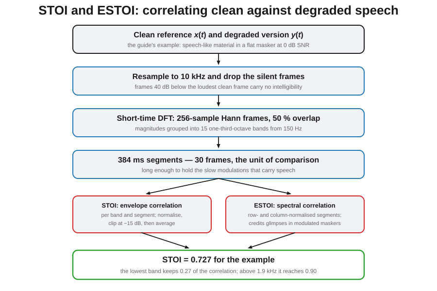
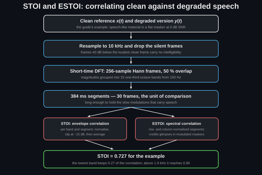
Section titled “1. The shared front end”Both measures run the same processing before they diverge (Taal et al. 2011, Section II): resampling to 10 kHz; a 256-sample (25.6 ms) Hann-windowed, 50 %-overlapping short-time transform zero-padded to 512 points; removal of the frames whose clean energy is more than 40 dB below the loudest clean frame; a 15-band one-third-octave grouping of the DFT magnitudes from a lowest centre of 150 Hz; and 384 ms (30-frame) analysis segments as the unit of comparison. The sample rate of the inputs is free, the library resamples internally.
Both measures are defined for running speech, and the front end is where that assumption bites: the 40 dB rule keys off the clean signal’s dynamic range, so it exists to stop the pauses between words from dominating the correlation. A signal with no pauses (steady noise, a held tone, gapless music) loses nothing to it and the index loses its meaning; a recording that is mostly silence loses almost everything and the call raises rather than returning a number. At least about 0.4 s of active speech has to survive.
import numpy as npfrom phonometry import speech
fs = 10000rng = np.random.default_rng(11)n = 4 * fst = np.arange(n) / fs
# Speech-like material: band-limited noise under a 3.5 Hz syllabic envelope,# so the front end's silent-frame rule has pauses to work on.spectrum = np.fft.rfft(rng.standard_normal(n))spectrum[(np.fft.rfftfreq(n, 1 / fs) < 200) | (np.fft.rfftfreq(n, 1 / fs) > 4000)] = 0carrier = np.fft.irfft(spectrum, n)clean = carrier * (0.15 + 0.85 * np.abs(np.sin(2 * np.pi * 3.5 * t)) ** 2)
noise = rng.standard_normal(n)noise *= np.sqrt(np.mean(clean ** 2) / np.mean(noise ** 2))   # 0 dB SNRdegraded = clean + noise
d = speech.stoi(clean, degraded, fs)               # STOI, resampled to 10 kHz insideprint(round(d.value, 3))                    # 0.708print(round(speech.stoi(clean, clean, fs).value, 6))   # 1.0  (a signal against itself)
Everything up to the 384 ms segments is shared; the two measures only part ways at the correlation. The diagram lays the chain out with the numbers of the flat-masker example.
Getting a valid pair
Section titled “Getting a valid pair”The two arguments are not just “two signals”. They must be the same utterance, the same length, and sample-accurate in alignment. That last one is the failure that costs most scores in practice, because nothing in the result distinguishes it from genuine degradation. Both measures correlate short-time envelopes inside 384 ms segments, so a constant delay decorrelates them directly. On the pair above, rolling the degraded signal by 20 ms takes the score from 0.708 to 0.329; on a perfect pair, the same 20 ms takes 1.0 to 0.459 and 50 ms drives it negative. Half a syllable is enough to turn a good enhancement into a bad one on paper.
The library enforces equal length and nothing else: it does no alignment, so
the caller compensates any algorithmic latency first. Cross-correlate the
broadband envelopes (or prepend a short marker chirp), shift, then trim both to
the common span. If the two signals passed through separate playback and
capture clocks, watch for drift as well: a fixed shift cannot correct a
sample-rate offset, so resample to the reference clock or record through one
device. The check worth running once on any new pipeline is the pair of lines
above: stoi(x, x, fs).value is 1.0, and stoi(x, np.roll(x, k), fs) collapses
quickly with k.
What you do not have to match is level: the per-segment normalisation makes both measures invariant to the gain of the degraded signal. Alignment is the thing to get right; gain is not.
Three conditions raise instead of returning a value, and they are worth recognising: unequal length, non-finite samples, and fewer than 30 short-time frames surviving the silent-frame removal, which is the ~0.4 s of active speech mentioned above.
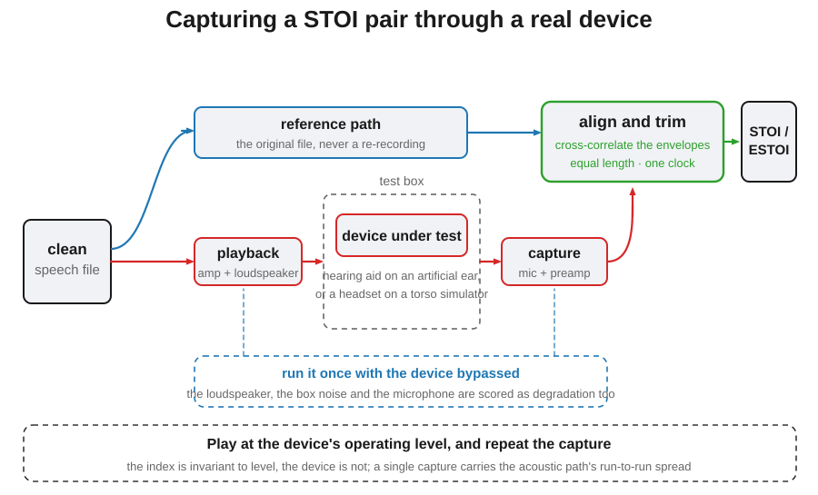
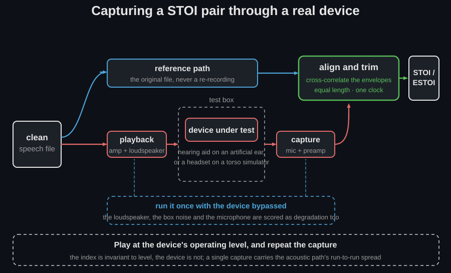
Capturing the degraded signal through a real device
Section titled “Capturing the degraded signal through a real device”Everything above assumes the degraded signal was produced numerically. Once it is captured acoustically (a hearing aid on an artificial ear in a test box, a headset, a loudspeaker-and-microphone loop), four things become the caller’s responsibility:
- The clean reference stays the original file. Re-recording it through the same chain removes the very distortion under test, and it also breaks the silent-frame selection, which is derived from the clean signal alone.
- The capture chain is scored as degradation. Loudspeaker response, background noise in the test box and microphone self-noise all enter the measured index, so measure the loop once with the device bypassed and report that number as the floor of the comparison.
- Play at the device’s operating level. The index is invariant to level; the device is not. A compressor or a noise reducer behaves differently at a different input level.
- Repeat. A single capture carries the run-to-run variability of the acoustic path; quote the spread over several captures, not one number.
2. STOI: envelope correlation with clipping
Section titled “2. STOI: envelope correlation with clipping”For every band and segment STOI normalises the degraded envelope to the clean one, clips it at a lower signal-to-distortion bound ( dB) so a fully degraded unit cannot drag the score below its floor, and takes the sample correlation of the two envelopes (Taal et al. 2011, Eqs. 3-6):
where is the clean short-time temporal envelope of band at frame inside the 30-frame segment ; is the degraded envelope after the per-segment gain normalisation and the dB clipping, so that accent marks the processing and not a mean; a bar over a whole quantity (, ) is its mean over the segment; and is the Euclidean norm over the same 30 frames. So is an ordinary Pearson correlation in .
The index is the average of those intermediate correlations over all bands
and segments (Eq. 6). The two marginals of that average are what
band_scores and segment_scores expose. Because the normalisation divides out a per-segment
gain, STOI is invariant to the overall playback level of the degraded
signal, and higher SNR gives a monotonically higher score.
from phonometry import speech
# The speech-like `clean` of section 1, degraded at four signal-to-noise# ratios. Keep the reference speech-like: a flat Gaussian reference has no# pauses, so the 40 dB rule removes nothing and the index loses its meaning.for snr_db in (-10, 0, 10, 20):    g = 10.0 ** (-snr_db / 20.0)    noisy = clean + g * rng.standard_normal(clean.size)    print(snr_db, round(speech.stoi(clean, noisy, fs).value, 3))# -10 0.083 | 0 0.484 | 10 0.858 | 20 0.956
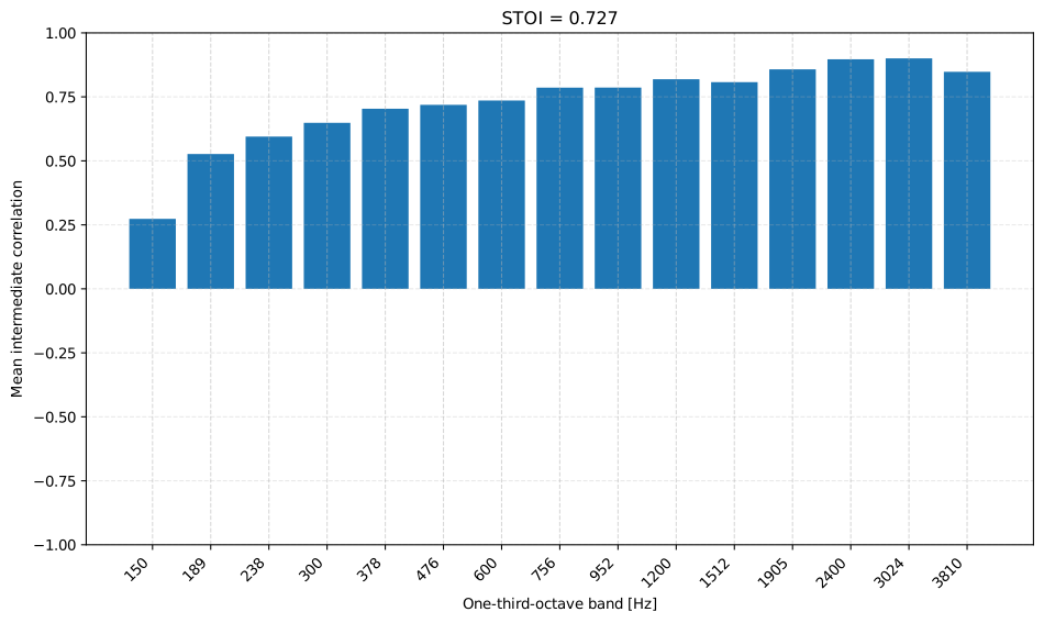
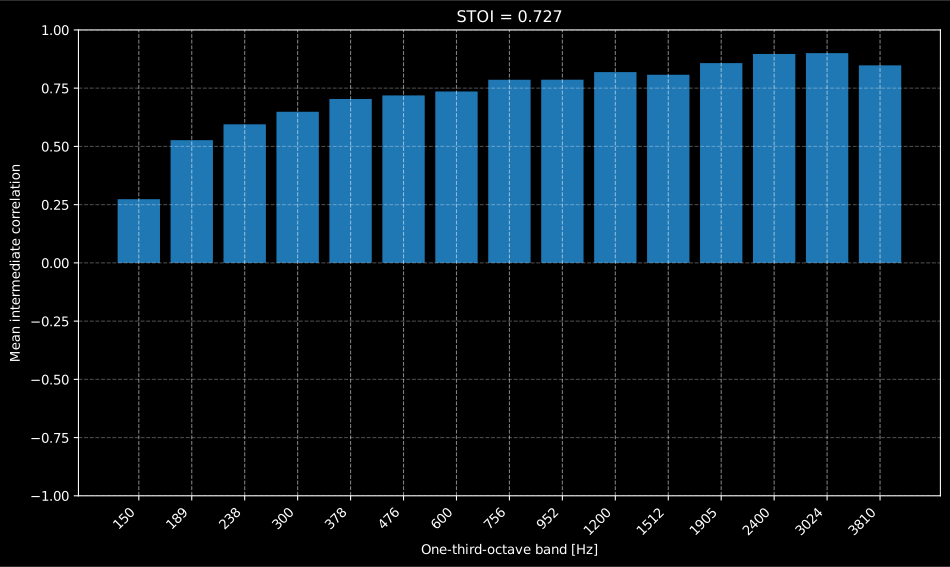
The STOIResult carries the per-band mean correlation (band_scores) and the
per-segment scores (segment_scores) that average to value, and its
.plot() draws the per-band intermediate correlation. That per-band view is
worth looking at before quoting the index: it shows where the degradation
bites, which the single number cannot.
Show the code for this figure
import numpy as npimport matplotlib.pyplot as pltfrom scipy.signal import butter, lfilterfrom phonometry import speech
# Speech-like material: band-limited noise with a 3.5 Hz syllabic envelope,# in a flat masker at 0 dB SNR.fs = 10000rng = np.random.default_rng(11)t = np.arange(4 * fs) / fsb, a = butter(2, [200 / (fs / 2), 4000 / (fs / 2)], btype="band")carrier = lfilter(b, a, rng.standard_normal(t.size))clean = carrier * (0.15 + 0.85 * np.abs(np.sin(2 * np.pi * 3.5 * t)) ** 2)masker = rng.standard_normal(clean.size)gain = np.sqrt(np.mean(clean ** 2)) / np.sqrt(np.mean(masker ** 2))res = speech.stoi(clean, clean + gain * masker, fs)print(round(res.value, 3))    # 0.727
# One line: the per-band intermediate correlation behind the index.res.plot()plt.show()
# By hand, mirroring what STOIResult.plot() draws:pos = np.arange(res.band_scores.size)fig, ax = plt.subplots()ax.bar(pos, res.band_scores)ax.set_xticks(pos)ax.set_xticklabels([f"{f:.0f}" for f in res.band_frequencies], rotation=45, ha="right")ax.set_xlabel("One-third-octave band [Hz]")ax.set_ylabel("Mean intermediate correlation")ax.set_title(f"STOI = {res.value:.3f}")plt.show()
The band profile is one marginal of the average; the other is time, and it answers a question the band view explicitly cannot:
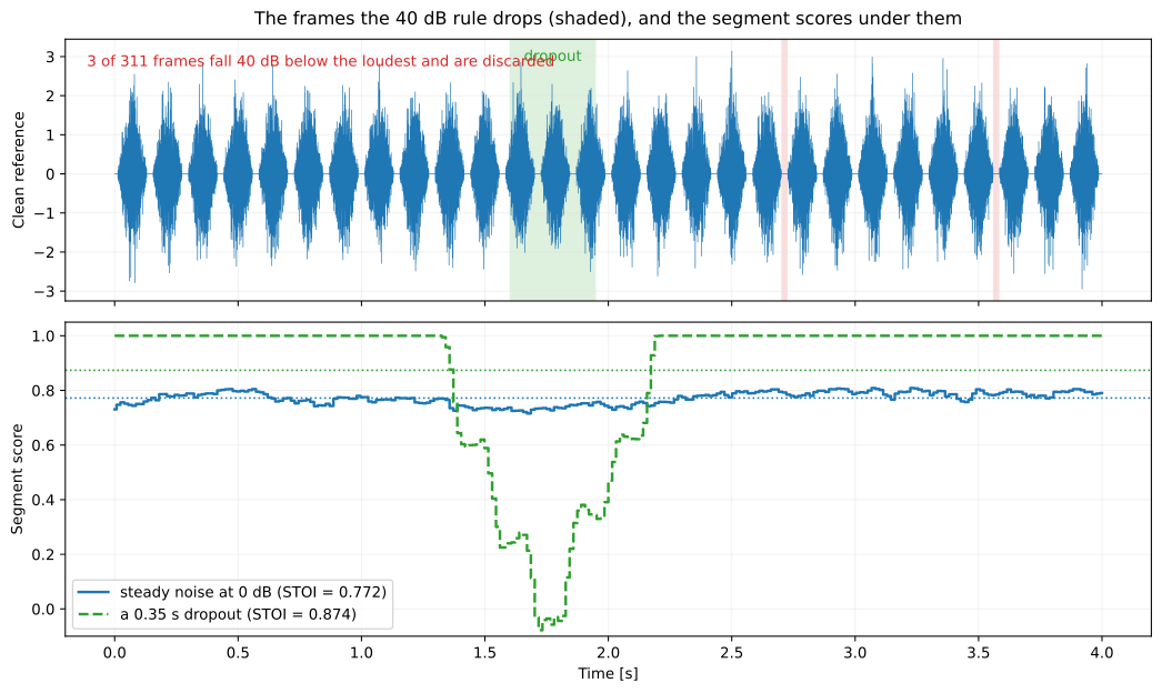
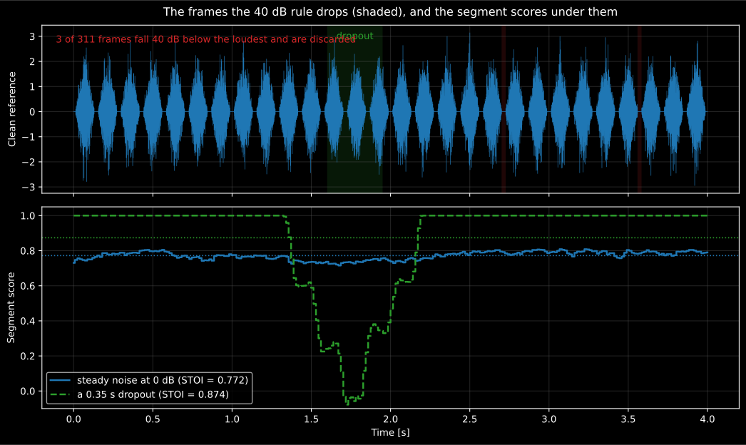
Two degradations of the same reference, and the scalar ranks them the wrong way round: the dropout scores 0.874 against the steady masker’s 0.772, because a short catastrophe averages away while a mild degradation everywhere does not. The time marginal separates them immediately: one series is flat, the other is perfect except for a handful of segments. That is the diagnostic to reach for when a low STOI has no obvious cause: a transient, a dropout or a processing artefact shows up here and nowhere else. The shaded frames at the top are the ones the 40 dB rule discards, which is what “the input must have speech dynamics” means concretely.
Show the code for this figure
# The same material as section 1 but with silence between the words, so some# frames really do fall 40 dB below the loudest one.fig_rng = np.random.default_rng(11)freq = np.fft.rfftfreq(n, 1 / fs)spec = np.fft.rfft(fig_rng.standard_normal(n))spec[(freq < 200) | (freq > 4000)] = 0env = np.abs(np.sin(2 * np.pi * 3.5 * t)) ** 2ref = np.fft.irfft(spec, n) * np.where(env < 0.08, 0.0, env)
masker = fig_rng.standard_normal(n)masker *= np.sqrt(np.mean(ref ** 2) / np.mean(masker ** 2))steady = speech.stoi(ref, ref + masker, fs)
hole = np.ones(n)hole[int(1.6 * fs):int(1.95 * fs)] = 0.0        # a 0.35 s dropoutdropout = speech.stoi(ref, ref * hole, fs)
print(round(steady.value, 3), round(dropout.value, 3))   # 0.772 0.874print(round(float(dropout.segment_scores.min()), 3))     # -0.078
The flat masker costs the low bands most, because the speech spectrum falls there while the masker does not, and the correlation recovers in the consonant-bearing bands above 1 kHz. A band profile that is flat, or that collapses only in one band, points at something other than broadband noise: a notch filter, a resonance, or a processing artefact of the enhancement under test.
3. ESTOI: spectral correlation for modulated maskers
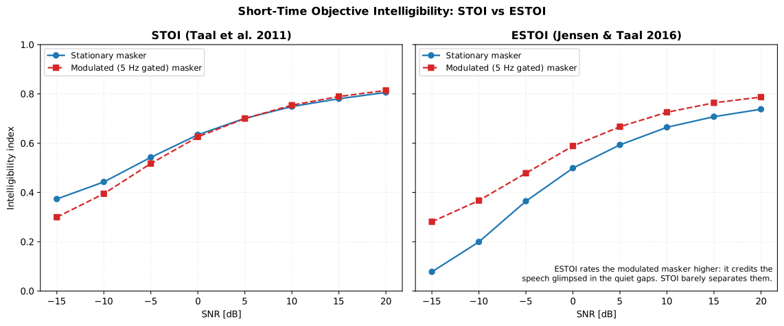
Section titled “3. ESTOI: spectral correlation for modulated maskers”ESTOI (extended=True) replaces the band-independent correlation with a joint
spectro-temporal one. Within each 384 ms segment it mean- and
variance-normalises the spectrogram rows (the band envelopes) and then its
columns (the per-frame spectra), and averages the correlation of the
normalised columns (Jensen and Taal 2016, Eqs. 4-8). Making the columns compete
means a masker that leaves quiet gaps, where the clean speech is briefly
audible, is credited for the speech glimpsed there, which STOI’s per-band
average largely misses.
Show the code for this figure
import numpy as npimport matplotlib.pyplot as pltfrom phonometry import speech
fs = 10000rng = np.random.default_rng(20)t = np.arange(3 * fs) / fs# A speech-like clean signal: amplitude-modulated formant-ish tones.clean = np.zeros_like(t)for f0 in (200.0, 400.0, 700.0, 1100.0, 1800.0, 2600.0):    depth = 0.5 * (1.0 + np.sin(2 * np.pi * rng.uniform(2.0, 6.0) * t + rng.uniform(0.0, 2 * np.pi)))    clean += depth * np.sin(2 * np.pi * f0 * t + rng.uniform(0.0, 2 * np.pi))p_clean = np.sqrt(np.mean(clean ** 2))
base = rng.standard_normal(clean.size)gate = 0.5 * (1.0 + np.sign(np.sin(2 * np.pi * 5.0 * t)))   # 5 Hz on/off gatemodulated = base * (0.05 + 0.95 * gate)snrs = np.arange(-15.0, 20.1, 5.0)
def curve(masker, extended):    p_m = np.sqrt(np.mean(masker ** 2))    return [speech.stoi(clean, clean + (p_clean / (p_m * 10.0 ** (s / 20.0))) * masker,                        fs, extended=extended).value for s in snrs]
fig, (a, b) = plt.subplots(1, 2, figsize=(12, 5), sharey=True)for ax, extended, title in ((a, False, "STOI"), (b, True, "ESTOI")):    ax.plot(snrs, curve(base, extended), "o-", label="Stationary masker")    ax.plot(snrs, curve(modulated, extended), "s--", label="Modulated masker")    ax.set_title(title); ax.set_xlabel("SNR [dB]"); ax.set_ylim(0, 1); ax.legend()a.set_ylabel("Intelligibility index")plt.show()
stoi() parameters
Section titled “stoi() parameters”| Parameter | Type | Units | Range / default | Notes |
|---|---|---|---|---|
clean | 1-D array | any | non-empty | The clean reference; the measure is level-invariant, so calibration is irrelevant |
degraded | 1-D array | any | same length as clean | Same utterance, same sample rate, sample-aligned |
fs | int | Hz | > 0 | Sample rate of both signals; resampled to 10 kHz internally |
extended | bool | — | default False | True selects ESTOI |
Returns a STOIResult: value, band_scores (15), segment_scores,
band_frequencies and extended. It raises on unequal lengths, on non-finite
input, and when fewer than 30 short-time frames survive the silent-frame
removal.
Reading the value
Section titled “Reading the value”The raw index has no absolute interpretation, and it is not meant to have one. The mapping from to a percentage of words understood is a logistic fitted to one corpus and one listener group (which the library deliberately does not implement). So the same predicts different scores for different material, and quoting “STOI = 0.73” as an intelligibility is a category error.
The working practice follows from that. Hold the material, the talkers, the alignment and the analysis length fixed, and report the difference between conditions (the ΔSTOI between a processor and its unprocessed input) together with the number of utterances it was averaged over, because single-utterance values scatter. Mind the shape as well: the index saturates near 1 for mild degradations and flattens at the low end, so an improvement from 0.85 to 0.90 is worth far more in intelligibility than one from 0.35 to 0.40: monotonic does not mean linear. And when two conditions score alike, the per-band and per-segment views are the diagnostics that say whether they got there the same way.
4. Which measure, and when
Section titled “4. Which measure, and when”| STOI | ESTOI | |
|---|---|---|
| Intermediate quantity | Per-band envelope correlation, clipped | Row- and column-normalised spectral correlation |
| Level invariance | Yes (per-segment normalisation) | Yes (per-row and per-column normalisation) |
| Stationary maskers | Well validated | Well validated |
| Modulated maskers, competing talkers | Underrates the glimpsing benefit | Tracks it |
| Cost | Lower | A little higher |
For additive stationary noise the two measures are interchangeable and STOI is the lighter default; when the interference fluctuates in time, or when comparing processors that reshape the speech in time and frequency, prefer ESTOI.
Both answer a narrower question than the two standardised speech metrics of the library, and the choice between the three families is really a choice of what you can measure. STOI and ESTOI need a clean reference and the degraded signal, so they belong to processing work: noise reduction, source separation, codecs, hearing-aid algorithms. The STI (IEC 60268-16) needs no clean reference, only the channel, so it is what rates a room or a public-address system. The SII (ANSI S3.5-1997) needs neither signal, only spectra, so it is what predicts audibility for a listener with a given hearing threshold. When more than one is available, they answer different questions rather than confirming each other: a processor can raise STOI while the room keeps the STI poor.
What this guide covers
Section titled “What this guide covers”Covered
Taal et al. 2011 (STOI) and Jensen & Taal 2016 (ESTOI), the two correlation-based measures
stoi()implements: the shared front end of 10 kHz resampling, 256-sample Hann frames, 15 one-third-octave bands, 384 ms segments and 40 dB silent-frame removal (Taal et al. 2011, Eqs. 1-4); the per-band envelope correlation and averaged index (Eqs. 5-6); and, withextended=True, the row- and column-normalisation of the spectrogram and the spectral-correlation index (Jensen & Taal 2016, Eqs. 4-8).Not covered
Taal et al. 2011 also fits a logistic function mapping the index to a predicted percentage of words understood, calibrated on specific listening-test corpora.
stoi()returns only , asSTOIResult.value, not that percentage: the API has no percent-correct output or fitted coefficients. The 2010 ICASSP paper is cited only as the short conference version of the same algorithm, adding nothing implemented beyond the 2011/2016 equations above.
References
Section titled “References”- Jensen, J., & Taal, C. H. (2016). An algorithm for predicting the intelligibility of speech masked by modulated noise maskers. IEEE/ACM Transactions on Audio, Speech, and Language Processing, 24(11), 2009-2022. https://doi.org/10.1109/TASLP.2016.2585878ESTOI: the row- and column mean- and variance-normalisation of the short-time spectrogram (Eqs. 4-7) and the spectral-correlation intermediate index (Eq. 8).
- Taal, C. H., Hendriks, R. C., Heusdens, R., & Jensen, J. (2010). A short-time objective intelligibility measure for time-frequency weighted noisy speech. 2010 IEEE International Conference on Acoustics, Speech and Signal Processing (ICASSP), 4214-4217. https://doi.org/10.1109/ICASSP.2010.5495701The short conference version of STOI.
- Taal, C. H., Hendriks, R. C., Heusdens, R., & Jensen, J. (2011). An algorithm for intelligibility prediction of time-frequency weighted noisy speech. IEEE Transactions on Audio, Speech, and Language Processing, 19(7), 2125-2136. https://doi.org/10.1109/TASL.2011.2114881STOI: the shared front end (10 kHz, 256-sample Hann frames, 15 one-third-octave bands, 384 ms segments), the normalisation and signal-to-distortion clipping (Eqs. 1-4), the per-band envelope correlation (Eq. 5) and the averaged index (Eq. 6).