Psychoacoustic annoyance and fluctuation strength

How annoying a sound is depends on more than how loud it is. Fastl & Zwicker, Psychoacoustics: Facts and Models, combine four psychoacoustic sensations (loudness, sharpness, roughness and fluctuation strength) into a single psychoacoustic annoyance $PA$, a scalar that grows with loudness and is lifted further when the sound is sharp, rough or slowly fluctuating. This page covers the exact $PA$ model (Eqs 16.2–16.4), the fluctuation strength it consumes, both the closed form for amplitude-modulated broadband noise (Eq. 10.2) and the Osses et al. (2016) signal model, and the signal convenience that derives all four sensations from a recording.

Show the code for this figure

import matplotlib.pyplot as plt
import numpy as np
from phonometry import psychoacoustics

n5 = np.linspace(4.0, 60.0, 200)
profiles = [
    ("Baseline: S = 1.75 acum, F = R = 0", 1.75, 0.0, 0.0),
    ("Sharp: S = 3.5 acum", 3.5, 0.0, 0.0),
    ("Rough + fluctuating: F = 1.2 vacil, R = 0.7 asper", 2.0, 1.2, 0.7),
]
fig, ax = plt.subplots()
for label, s, f, r in profiles:
    pa = [psychoacoustics.psychoacoustic_annoyance(v, s, f, r).annoyance for v in n5]
    ax.plot(n5, pa, label=label)

ex = psychoacoustics.psychoacoustic_annoyance(30.0, 2.0, 0.5, 0.3)
ax.plot([30.0], [ex.annoyance], "o", label=f"Worked example (PA = {ex.annoyance:.2f})")
ax.set_xlabel("Percentile loudness N5 [sone]")
ax.set_ylabel("Psychoacoustic annoyance PA")
ax.legend()
plt.show()

1. The four sensations

Psychoacoustic annoyance rests on four hearing sensations, each with its own model and unit in the library:

• Loudness: the percentile loudness $N_5$ (the loudness exceeded 5 % of the time), in sone, from the ISO 532-1 Zwicker time-varying model (loudness_zwicker, see Loudness).
• Sharpness $S$, in acum: the spectral balance towards high frequencies, DIN 45692 (sharpness_din).
• Roughness $R$, in asper: the harshness of fast (~70 Hz) amplitude modulation, ECMA-418-2 Sottek model (roughness_ecma).
• Fluctuation strength $F$, in vacil: the sensation of slow (~4 Hz) loudness fluctuation (§3 below).

2. Psychoacoustic annoyance (Eqs 16.2–16.4)

The exact model (Fastl & Zwicker Eq. 16.2; origin Widmann 1992) scales $N_5$ by a factor that grows with the sharpness weighting $w_S$ and the combined roughness/fluctuation weighting $w_{FR}$:

$$PA=N_5\left(1+\sqrt{w_S^2+w_{FR}^2}\right),w_S=(S-1.75)0.25{\log }_{10}(N_5+10)(S>1.75\mathrm{acum}),w_{FR}=\frac{2.18}{N_5^{0.4}}(0.4F+0.6R).$$

$w_S$ is zero for $S\le 1.75\text{acum}$ (sharpness only adds annoyance above that threshold); $w_{FR}$ weights roughness more heavily than fluctuation strength (0.6 vs 0.4). Those two choices are the whole of the modelling judgement in the formula, and they are easier to trust once seen:

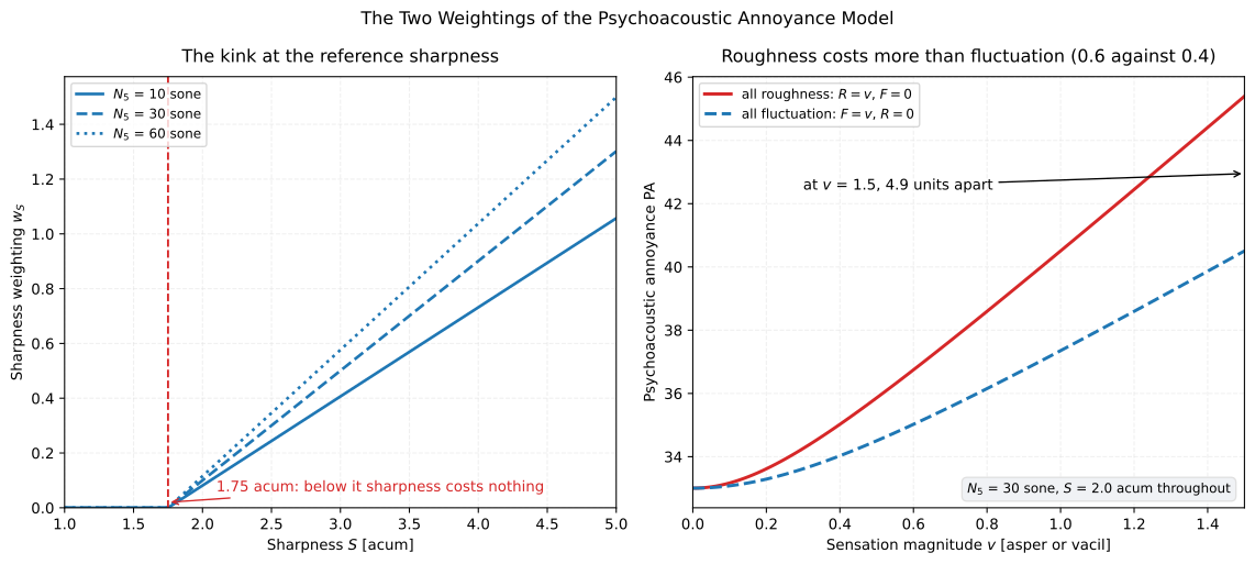
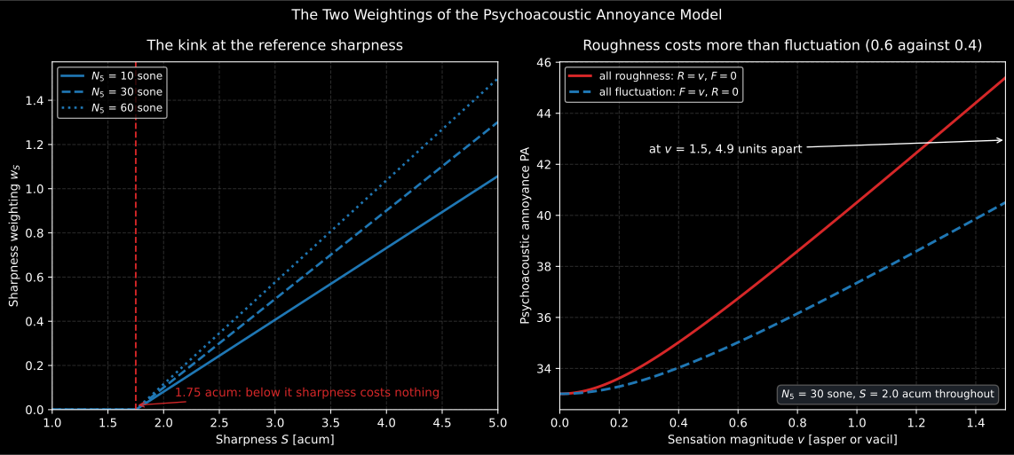
A sound has to be sharper than the 1.75 acum reference before sharpness costs anything at all, and the fan above that point is the loudness dependence of $w_S$. On the right, the same sensation magnitude buys about half again as much annoyance when it arrives as roughness rather than as fluctuation strength.

Show the code for this figure

import matplotlib.pyplot as plt
import numpy as np

# `psychoacoustics` is imported by the snippet above.
sharpness = np.linspace(1.0, 5.0, 200)
for n5 in (10.0, 30.0, 60.0):
    w_s = [psychoacoustics.psychoacoustic_annoyance(n5, float(s), 0.0, 0.0).w_s
           for s in sharpness]
    plt.plot(sharpness, w_s, label=f"N5 = {n5:g} sone")
plt.axvline(1.75, linestyle="--")
plt.xlabel("Sharpness S [acum]")
plt.ylabel("Sharpness weighting wS")
plt.legend()
plt.show()

# The same magnitude spent on roughness or on fluctuation strength, at a
# fixed N5 = 30 sone and S = 2.0 acum:
rough = psychoacoustics.psychoacoustic_annoyance(30.0, 2.0, 0.0, 1.5).annoyance
fluct = psychoacoustics.psychoacoustic_annoyance(30.0, 2.0, 1.5, 0.0).annoyance
print(round(rough, 1), round(fluct, 1))   # 45.4 40.5

psychoacoustic_annoyance takes the four quantities directly and returns the annoyance together with the two intermediate weightings:

from phonometry import psychoacoustics

res = psychoacoustics.psychoacoustic_annoyance(30.0, 2.0, 0.5, 0.3)   # N5, S, F, R
print(round(res.annoyance, 4))   # 37.0477
print(round(res.w_s, 4), round(res.w_fr, 4))   # 0.1001 0.2125

res.plot()   # PA beside its wS and wFR weightings (needs matplotlib)

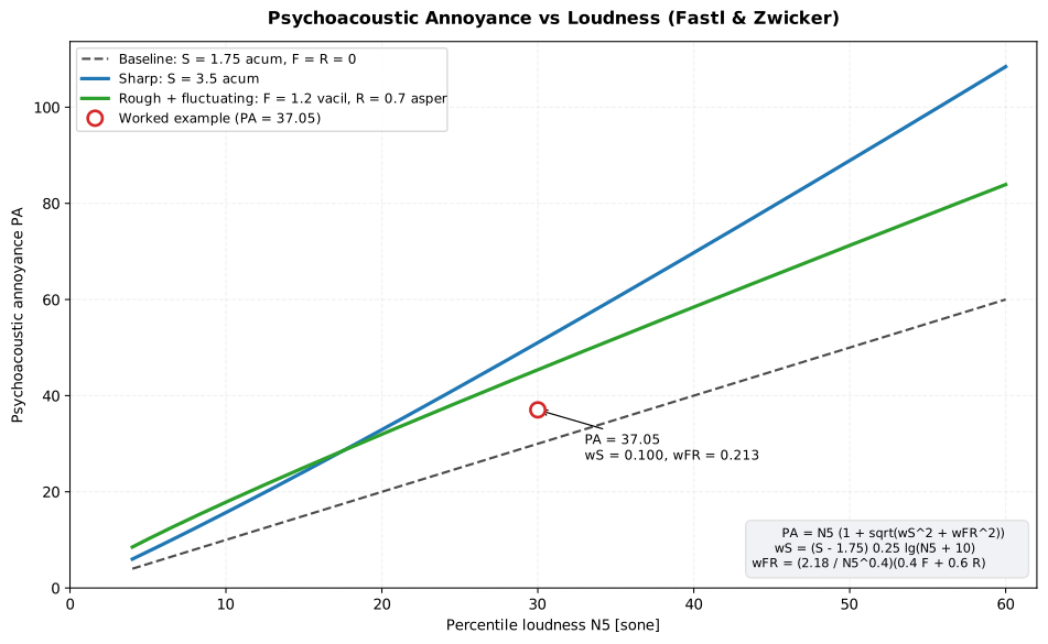
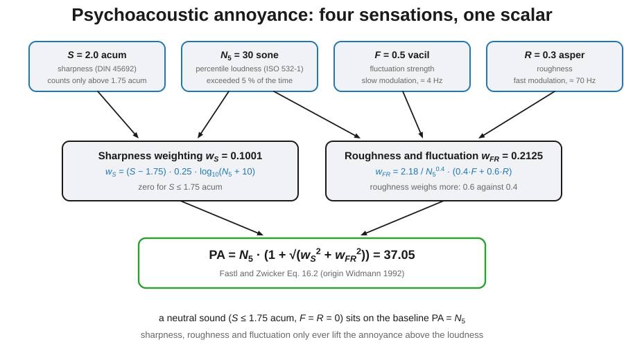
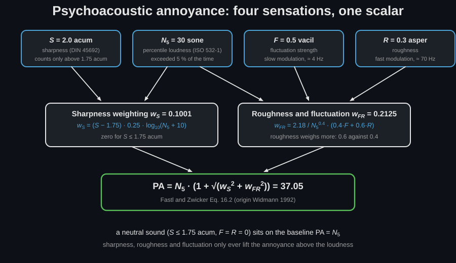
What that number means. $PA$ carries no unit and no criterion. It is built so that a neutral sound — sharpness at or below 1.75 acum, no roughness, no fluctuation — has a $PA$ equal to its $N_5$ in sone, and every sharp, rough or fluctuating quality can only push it above that floor. So read $PA$ as “the loudness this sound is worth once its character is taken into account”: the worked example’s 37.05 against an $N_5$ of 30 sone says the character costs 23 %. Comparison is the point — rank two designs of the same product, or quantify what a fix bought — and no limit exists to quote it against.

Caution

This is not the annoyance of environmental-noise assessment. Psychoacoustic annoyance is a laboratory scaling of a single sound. It says nothing about long-term exposure, time of day, the attitude of the population towards the source, or the percentage highly annoyed, which is the business of the rating levels and exposure-response relations in Environmental Levels. A $PA$ of 37 is not “37 % highly annoyed”, and the two quantities are not convertible.

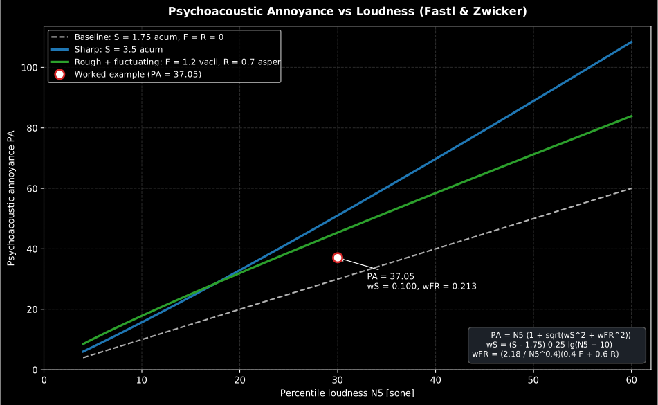
The figure above sweeps $PA$ against $N_5$ for three profiles: a neutral baseline ($S=1.75\text{acum}$, $F=R=0$, so $PA=N_5$), a sharp sound and a rough-and-fluctuating sound, both lifted above the baseline, with the worked example marked.

The model is small enough to draw whole: two weightings and one combination. The diagram traces the worked example through it, sensation by sensation.

2.1 From a signal (engineering estimate)

psychoacoustic_annoyance_from_signal is a convenience that derives all four sensations from a calibrated pressure signal and combines them: $N_5$ from the ISO 532-1 Zwicker time-varying loudness, $S$ from DIN 45692 sharpness, $R$ from the ECMA-418-2 Sottek roughness and $F$ from the fluctuation-strength signal model.

The convenience is only as good as the record it is given, and neither entry point on this page takes a calibration argument, so x must already be calibrated pressure in pascals — see Measuring the input on the loudness page for how that factor is obtained. Beyond calibration: unweighted; one declared operating state rather than a run-up; long enough that $N_5$ is a percentile of something and that the ~4 Hz fluctuation analysis has enough modulation periods, which in practice means several seconds and the same length for every design being compared; and field= matching how the sound was captured. A two-second clip yields an $N_5$ that is nearly $N_{\text{max}}$ and an $F$ biased low. A binaural or artificial-head recording is analysed one ear at a time, already equalized to the free or diffuse field, and the louder channel is the one usually reported.

import numpy as np
from phonometry import psychoacoustics

# A raw recording plus its calibration so the guide runs standalone. There is
# no calibration_factor argument here, so x must already be in pascals.
fs = 48000
t = np.arange(int(5.0 * fs)) / fs
x = (1.0 + 0.8 * np.sin(2 * np.pi * 4.0 * t)) * np.sin(2 * np.pi * 1000 * t)
x *= 2e-5 * 10 ** (70 / 20) / np.sqrt(np.mean(x**2))   # calibrated to 70 dB SPL

res = psychoacoustics.psychoacoustic_annoyance_from_signal(x, fs, field="free")
print(f"PA = {res.annoyance:.1f}  (N5 = {res.n5:.1f} sone, S = {res.sharpness:.2f} acum,"
      f" R = {res.roughness:.2f} asper, F = {res.fluctuation_strength:.2f} vacil)")

res.plot()   # the same PA / wS / wFR view, now from the four derived sensations

All four sensations must come from the same record and the same operating state: PA is a combination rule, not a measurement in its own right, so computing $N_5$ over a minute and $R$ over two seconds of it silently mixes two different sounds. Quote each sensation with the model that produced it.

Caution

Model-mixing caveat. This composite mixes model families: Zwicker-family $N_5$ and $S$, Sottek $R$ and Osses $F$. The $PA$ model was calibrated with Zwicker-family sensations, so treat the signal convenience as an engineering estimate. For exact, reproducible results, compute the four quantities with whichever models you trust and pass them to psychoacoustic_annoyance directly (the four-argument function is the exact model).

3. Fluctuation strength

Fluctuation strength $F$ (vacil) quantifies the perception of slow loudness fluctuation. Like roughness it is a band-pass sensation of the modulation frequency, but it peaks about an order of magnitude lower, at $f_{mod}\approx 4\text{Hz}$ rather than the ~70 Hz roughness peak. By definition, a 1 kHz tone at 60 dB, 100 % amplitude-modulated at 4 Hz, produces 1 vacil. This page covers two of the three fluctuation-strength models in the library: the Fastl & Zwicker closed form for amplitude-modulated broadband noise (§3.1) and the Osses et al. (2016) signal model for arbitrary signals (§3.2). The normative Sottek-model fluctuation strength of ECMA-418-2 Clause 9, in vacil_HMS, lives in Sound Quality Metrics — note that this page’s unit is the vacil and that one the vacil_HMS, so the two are not the same number for the same sound.

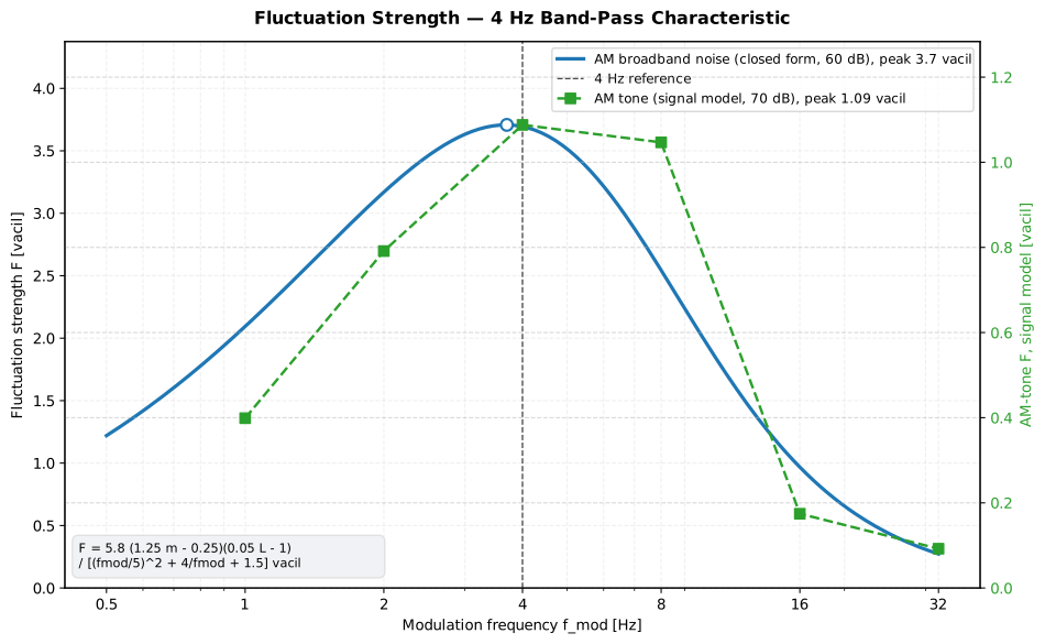
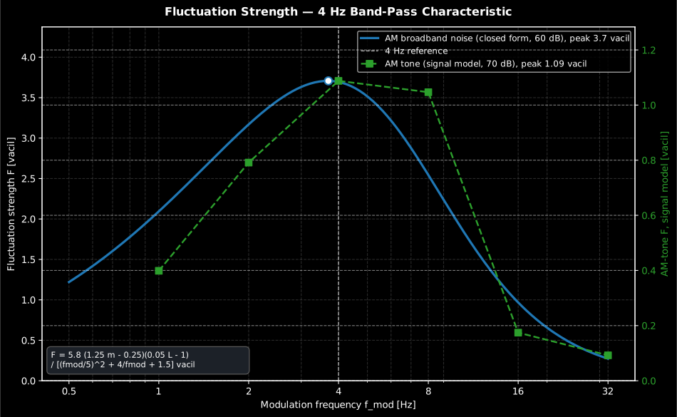
The two models on the same stimulus, which is the comparison the caution box below turns into a rule. Both are band-passes centred near 4 Hz, but on AM broadband noise the signal model overshoots the closed form by about half again, because it accumulates modulation band by band across the whole Bark axis. On the AM tone it was calibrated for, right, it behaves.

Show the code for this figure

import matplotlib.pyplot as plt
import numpy as np
from phonometry import psychoacoustics

# Left panel, the two models on the same stimulus: AM broadband noise at
# 60 dB, 100 % modulation.
fmod = np.logspace(np.log10(0.5), np.log10(32.0), 240)
f_bbn = [psychoacoustics.fluctuation_strength_am_noise(60.0, 1.0, fm) for fm in fmod]

rng = np.random.default_rng(3)
tn = np.arange(int(4.0 * fs)) / fs
noise = rng.standard_normal(tn.size)
fm_noise = [0.5, 1.0, 2.0, 4.0, 8.0, 16.0, 32.0]
f_noise = []
for fm in fm_noise:
    am = (1.0 + np.sin(2 * np.pi * fm * tn)) * noise
    am = am / np.sqrt(np.mean(am ** 2)) * 2e-5 * 10 ** (60 / 20)
    f_noise.append(psychoacoustics.fluctuation_strength(am, float(fs)).fluctuation_strength)
print(round(f_noise[3], 1), round(f_bbn[np.argmin(np.abs(fmod - 4.0))], 1))   # 5.5 3.7

fig, ax = plt.subplots()
ax.semilogx(fmod, f_bbn, label="closed form, Eq. 10.2")
ax.semilogx(fm_noise, f_noise, "s--", label="Osses 2016 signal model")
ax.axvline(4.0, ls="--", color="0.4")
ax.set_xlabel("Modulation frequency f_mod [Hz]")
ax.set_ylabel("Fluctuation strength F [vacil]")
ax.legend(loc="upper right")
plt.show()

3.1 Closed form for AM broadband noise (Eq. 10.2)

For sinusoidally amplitude-modulated broadband noise, Fastl & Zwicker give a closed form (Eq. 10.2) in modulation factor $m$, level $L$ and modulation frequency $f_{mod}$:

$$F=\frac{5.8(1.25m-0.25)[0.05(L/\mathrm{dB})-1]}{(f_{mod}/5\mathrm{Hz}{)}^2+(4\mathrm{Hz}/f_{mod})+1.5}\mathrm{vacil}.$$

The denominator is the 4 Hz band-pass: it bottoms out near $f_{mod}\approx 3.7\text{Hz}$ and rises on either side. The result is clamped at 0 (the sensation vanishes below ~20 dB or $m<0.2$). This exact form is the value to quote for AM broadband noise.

from phonometry import psychoacoustics

print(round(psychoacoustics.fluctuation_strength_am_noise(60.0, 1.0, 4.0), 4))   # 3.6943 vacil

3.2 The Osses 2016 signal model

fluctuation_strength implements the Osses et al. (2016) signal model: it builds an excitation pattern over 47 auditory filters, extracts the ~4 Hz envelope modulation per band, weights and combines it, and returns the overall $F$ (vacil) plus the specific fluctuation strength over the Bark axis and the time-dependent trace.

from phonometry import psychoacoustics

res = psychoacoustics.fluctuation_strength(x, fs)
print(round(res.fluctuation_strength, 2))   # 0.65 vacil for the signal above
res.plot()   # specific fluctuation strength F′(z) over the Bark axis (needs matplotlib)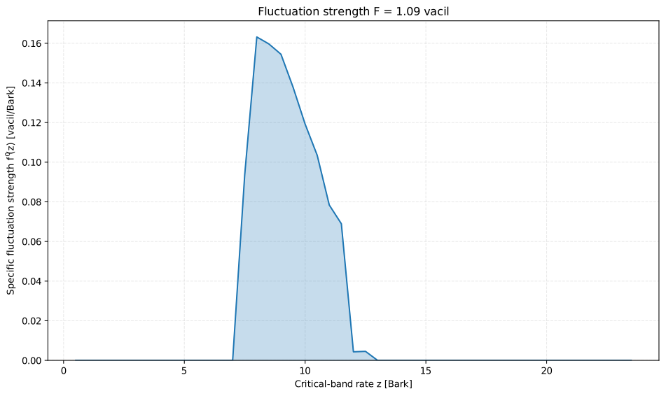

Show the code for this figure

import matplotlib.pyplot as plt
import numpy as np
from phonometry import psychoacoustics

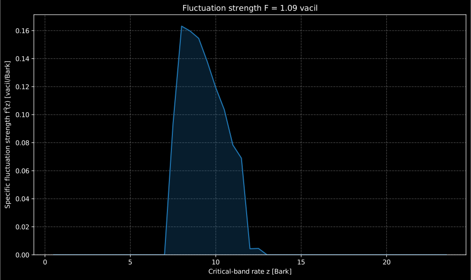
# The reference-like stimulus: a 1 kHz tone at 70 dB SPL, 100 % amplitude
# modulated at 4 Hz, where the sensation peaks.
fs = 48000
t = np.arange(int(2.0 * fs)) / fs
am = (1.0 + np.sin(2 * np.pi * 4.0 * t)) * np.sin(2 * np.pi * 1000 * t)
am = am / np.sqrt(np.mean(am ** 2)) * 2e-5 * 10 ** (70 / 20)
res = psychoacoustics.fluctuation_strength(am, float(fs))
print(round(res.fluctuation_strength, 2))    # 1.09 vacil

# One line: the specific fluctuation strength over the Bark axis.
res.plot()
plt.show()

# Or draw f'(z) by hand from the arrays the result carries:
fig, ax = plt.subplots()
ax.fill_between(res.bark_axis, res.specific, alpha=0.3)
ax.plot(res.bark_axis, res.specific)
ax.set_xlabel("Critical-band rate z [Bark]")
ax.set_ylabel("Specific fluctuation strength [vacil/Bark]")
plt.show()

The sensation stays where the modulated energy is, in the critical bands around the carrier, which is exactly why the closed form of §3.1 and the signal model diverge for broadband modulated noise: there the modulation is spread over the whole Bark axis and the band-by-band model accumulates more of it than the single closed form allows.

Note

No numeric standard. Fluctuation strength has no ISO/IEC standard. This is a clean-room implementation from the Osses 2016 paper, calibrated so that the 1 kHz / 60 dB / $m=1$ / 4 Hz AM tone reads 1.00 vacil by construction, and cross-checked against the Osses 2016 Table 1 literature values and the open SQAT reference (used only as a numeric oracle). Over the 70 dB AM-tone sweep $f_{mod}\in \{1,2,4,8,16,32\}\text{Hz}$ it gives [0.40, 0.79, 1.09, 1.05, 0.17, 0.09] vacil against the literature [0.39, 0.84, 1.25, 1.30, 0.36, 0.06] (Pearson $r=0.98$, correct 4 Hz peak, within ~2.1×). FM-tone accuracy is explicitly not pursued. For AM broadband noise the signal model overshoots the absolute level (it spreads the modulated energy across bands); quote the closed form fluctuation_strength_am_noise (§3.1) for that stimulus.

What this guide covers

• Covered

  Fastl & Zwicker’s Psychoacoustics: Facts and Models gives the exact $PA$ model, Eqs 16.2-16.4 (origin Widmann 1992), run by psychoacoustic_annoyance. It also gives the closed form for AM broadband noise, Eq. 10.2, run by fluctuation_strength_am_noise. The Osses et al. (2016) signal model for fluctuation strength runs as fluctuation_strength, cross-checked against its Table 1 literature values and the SQAT reference. psychoacoustic_annoyance_from_signal derives the four inputs from a signal (ISO 532-1 Zwicker $N_5$, DIN 45692 $S$, ECMA-418-2 $R$) and combines them with the exact model.

• Not covered

  The Osses 2016 model’s accuracy for FM tones is explicitly not pursued. Only AM stimuli are validated here. The front-end also departs from the paper’s exact framing (2 s frames, 90 % overlap, absolute-threshold gating). As a result, a steady 1 kHz tone reads about 0.09 vacil instead of 0, and steady broadband noise reads about 0.15-0.19 vacil. For AM broadband noise, quote fluctuation_strength_am_noise (§3.1) instead of fluctuation_strength, which overshoots that stimulus. The normative Sottek-model fluctuation strength of ECMA-418-2 Clause 9 is not implemented on this page: it lives in Sound Quality Metrics.

See also

• Loudness: the ISO 532-1 percentile loudness $N_5$ this model takes as its first argument, and the acquisition rules the recording has to satisfy before any of it applies.
• Sound Quality Metrics: the DIN 45692 sharpness $S$, the ECMA-418-2 roughness $R$ and the normative vacil_HMS fluctuation strength of the same sensation this page models in vacil.
• Advanced Loudness: the alternative loudness models, and why mixing families makes the composite an engineering estimate.
• Environmental Levels: community annoyance, the other thing the word means, and the rating levels it is assessed with.
• Theory: Advanced loudness models and sound quality: the loudness and sound-quality metrics the annoyance model combines, derived one at a time.
• API reference: psychoacoustics.quality.annoyance and psychoacoustics.quality.fluctuation_strength.

References

• Fastl, H., & Zwicker, E. (2007). Psychoacoustics: Facts and models (3rd ed.). Springer. https://doi.org/10.1007/978-3-540-68888-4The source of the psychoacoustic-annoyance model of section 2 (Eqs 16.2-16.4, chapter 16; origin Widmann 1992) and of the closed-form fluctuation strength for AM broadband noise of section 3.1 (Eq. 10.2, chapter 10).
• Felix Greco, G., Merino-Martínez, R., Osses, A., & Lotinga, M. J. B. (2025). SQAT: A sound quality analysis toolbox for MATLAB. GitHub. https://doi.org/10.5281/zenodo.7934709The open MATLAB reference (open-source software) used as the numeric oracle for the fluctuation-strength cross-checks on this page.
• Osses Vecchi, A., García León, R., & Kohlrausch, A. (2016). Modelling the sensation of fluctuation strength. Proceedings of Meetings on Acoustics, 28, 050005. https://doi.org/10.1121/2.0000410The fluctuation-strength signal model implemented in section 3.2 (presented at ICA 2016; clean-room, with no numeric standard, calibrated to 1 vacil at the reference AM tone), including the Table 1 literature values used as its cross-check.