Hearing Protectors (ISO 4869-1, -2 and -6)

A hearing protector is not measured on a coupler. ISO 4869-1 seats it on sixteen people and records the threshold shift each of them gets, so what comes back from the laboratory is a distribution: one attenuation per subject per octave band, with a spread that is often a third of the mean. ISO 4869-2 is the standard that turns that distribution into a number someone can act on, and the first thing it does is refuse to use the mean.

ISO 4869-1 measures the attenuation at the threshold of hearing. The test signals are one-third-octave bands of pink noise centred on the octave frequencies from 125 Hz to 8 kHz, with 63 Hz optional (4.1). Each of sixteen subjects finds a threshold for every one of them twice, with open ears and with the protector in place, half the panel in each order, and the attenuation of that subject in that band is the difference (4.6.2):

A report gives those individual values and, per test signal, their mean, their standard deviation and the expanded uncertainty of the mean (Clause 6). Annex A models the attenuation as the measured value plus three zero-mean inputs, for the method (the subject group, the fitting, the threshold judgement, the tester, the specimen), the test equipment and the environment. Within one laboratory the combined standard uncertainty of a given measurement is the standard deviation of its mean, and the coverage factor is 2:

import numpy as np
from phonometry import hearing

# ISO 4869-1 Table A.3: one earmuff on sixteen subjects, 125 Hz to 8 kHz.
table_a3 = np.array([
    [9.6, 13.5, 27.5, 32.4, 35.2, 29.1, 28.5],  [14.1, 20.2, 25.8, 32.0, 28.9, 35.3, 35.7],
    [21.8, 27.8, 28.3, 46.6, 37.4, 40.1, 38.7], [18.5, 22.2, 36.5, 44.8, 39.1, 30.6, 33.5],
    [15.6, 21.9, 31.8, 42.5, 38.9, 38.3, 37.1], [18.7, 28.6, 31.3, 39.0, 35.6, 35.3, 29.4],
    [23.0, 26.5, 34.0, 41.3, 40.8, 38.7, 35.9], [17.3, 21.7, 25.0, 30.7, 38.6, 37.9, 40.8],
    [19.4, 19.6, 28.0, 36.6, 40.7, 34.9, 39.4], [11.6, 20.4, 22.6, 38.0, 39.2, 33.9, 30.3],
    [20.5, 21.8, 29.2, 40.7, 36.2, 35.7, 38.4], [18.3, 19.6, 26.2, 34.6, 32.7, 34.9, 26.6],
    [15.1, 17.5, 30.1, 39.0, 39.4, 38.2, 39.5], [21.7, 20.8, 28.3, 39.5, 38.1, 40.0, 38.4],
    [15.9, 17.8, 26.0, 40.6, 38.0, 40.2, 37.2], [11.8, 18.4, 29.6, 37.2, 40.8, 36.0, 29.9],
])
reat = hearing.real_ear_attenuation(table_a3)
print(np.round(reat.mean_db, 1))                  # [17.1 21.1 28.8 38.5 37.5 36.2 35. ]
print(np.round(reat.standard_deviation_db, 1))    # [3.9 3.9 3.5 4.5 3.2 3.2 4.6]
print(np.round(reat.expanded_uncertainty_db, 1))  # [2.  1.9 1.7 2.2 1.6 1.6 2.3]

# The grid is the input of every ISO 4869-2 method below, unchanged.
print(np.round(hearing.assumed_protection_value(reat.attenuation_db).apv, 1))
# [13.1 17.2 25.3 34.  34.3 33.  30.4]

The thresholds themselves can go in instead, as open_threshold_db and occluded_threshold_db; they only need to share a reference, since a level in sound pressure and one in hearing level give the same difference. Everything is computed at full precision and rounded by whoever prints it, which is what Tables A.3 and B.1 say they do.

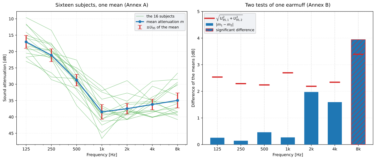
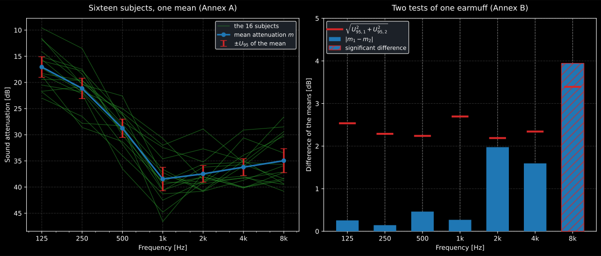
Left, Table A.3: the spread across subjects is several decibels, and the expanded uncertainty of the mean drawn on it is half that spread, because sixteen subjects divide it by four and the coverage factor doubles it back. Right, Table B.1: two tests of the earmuff under two test conditions (for example two headband positions), which differ by more than the two uncertainties allow only at 8 kHz.

import matplotlib.pyplot as plt

# One line each, from the results computed on this page.
reat.plot()          # mean downwards, subjects faint, U95 as bars (Clause 6 l))
plt.show()

test_2_mean = [16.8, 21.0, 28.3, 38.2, 35.5, 34.6, 38.9]
test_2_u95 = [1.6, 1.2, 1.4, 1.5, 1.5, 1.7, 2.5]
hearing.assess_attenuation_difference(
    reat, test_2_mean, second_expanded_uncertainty_db=test_2_u95
).plot()
plt.show()

Two mean attenuations differ significantly at the 5 % level when their difference exceeds the root sum of squares of their expanded uncertainties (B.1.2):

Table B.1 applies it to the earmuff above and to a second test of it under another test condition (headband position is the example B.1.2 gives), which the standard prints only as means and uncertainties:

test_2_mean = [16.8, 21.0, 28.3, 38.2, 35.5, 34.6, 38.9]
test_2_u95 = [1.6, 1.2, 1.4, 1.5, 1.5, 1.7, 2.5]
difference = hearing.assess_attenuation_difference(
    reat, test_2_mean, second_expanded_uncertainty_db=test_2_u95
)
print(np.round(difference.criterion_db, 1))  # [2.5 2.3 2.2 2.7 2.2 2.3 3.4]
print(difference.significant_frequencies)    # [8000.]

When there are no data of the specific measurement, B.1.1 and B.2 take the typical uncertainties of Table A.2 (within one laboratory) and Table B.2 (between laboratories), for earplugs and earmuffs in three frequency ranges. The library carries the three components of each and derives the combined and expanded values from them, which reproduces every printed cell. For two equal uncertainties the criterion becomes $\sqrt{2}{U}_{95}$, and B.1.1 evaluates it on the rounded value its table prints, writing that input out: ”$\sqrt{2}$ × 2,3 dB = 3,3 dB”. The unrounded budget gives 3.21 dB:

plug = hearing.REAT_WITHIN_LABORATORY_UNCERTAINTY["earplug"]["250 Hz up to 4 kHz"]
print(round(plug.expanded_db, 2))                                          # 2.27
print(round(hearing.minimum_significant_difference(2.3), 1))               # 3.3
print(round(hearing.minimum_significant_difference(plug.expanded_db), 2))  # 3.21

# The typical U95 band by band, ready for assess_attenuation_difference.
print(np.round(hearing.reat_expanded_uncertainty(reat.frequencies, protector="earplug"), 1))
# [3.2 2.3 2.3 2.3 2.3 2.3 3.2]

Between laboratories the same earplug needs 9.3 dB by B.2’s arithmetic ($\sqrt{2}$ × 6.6 dB), or 9.37 dB from the unrounded 6.62 dB: two laboratories disagree mostly on how their subjects fit the protector.

The sound field is qualified with the subject and the chair absent. The level 15 cm from the reference point on the three axes stays within ±2.5 dB of the level at it, the right and left positions within 3 dB of each other, and from 500 Hz up a directional microphone rotated through 360° sees a variation no larger than Table 1 allows for its free-field rejection (20 dB from a rejection of 25 dB down to 5 dB for one of 10 dB, and no microphone below that):

field = hearing.check_reat_sound_field(
    {"front": [0.8] * 7, "back": [-0.6] * 7, "left": [1.1] * 7,
     "right": [-1.2] * 7, "up": [1.9] * 7, "down": [-2.0] * 7},
    [0.0] * 7,
    rotation_levels_db=[[0.0] * 7, [4.0] * 7],
    free_field_rejection_db=17.0,
)
print(hearing.allowable_field_variation(17.0))  # 10.0
print(field.passes)                             # True

4.2.2 b) is a requirement of the clause, not an extra: left out, the rotation leaves field.directionality_judged false and field.passes false with it, while field.uniform and field.balanced still give the verdict of a) band by band.

All three methods take a mean less a multiple of its own spread, and differ in what they take it over. The octave-band method takes it over the attenuations of each band, and the result is the assumed protection value:

$\alpha$ is the inverse standard normal cumulative distribution at the protection performance $x$ (Table 1), so $AP{V}_{f84}$ with $\alpha =1$ is the attenuation 84 % of wearers reach or beat, and $AP{V}_{f98}$ with $\alpha =2$ is what all but one in fifty reach. Quoting a protector at its mean would describe a wearer who does not exist.

The HML and SNR methods never form that value. They rate each subject first, against the eight reference noises of Table 2 or the pink noise of Table 3, and take the same reduction over those ratings (Formulae (3) to (5) and (19)). What the three share is the choice of $x$ and its $\alpha$.

import numpy as np
from phonometry import hearing

# ISO 4869-1 attenuation of one protector: 16 subjects, eight octave bands
# from 63 Hz to 8 kHz. Annexes A to D of ISO 4869-2 work this same example
# through all three methods.
attenuation = np.array([
    [4, 8, 13, 18, 20, 30, 35, 30],   [6, 12, 16, 21, 29, 35, 47, 35],
    [10, 16, 17, 23, 25, 32, 48, 37], [3, 7, 12, 18, 20, 25, 33, 30],
    [8, 10, 16, 16, 25, 27, 43, 32],  [4, 7, 10, 15, 19, 32, 35, 31],
    [5, 5, 9, 16, 20, 25, 30, 28],    [15, 15, 21, 26, 25, 38, 46, 38],
    [5, 6, 10, 13, 19, 22, 29, 28],   [9, 9, 10, 19, 20, 27, 37, 31],
    [9, 16, 18, 24, 25, 35, 44, 39],  [5, 6, 11, 12, 17, 20, 28, 28],
    [7, 10, 17, 22, 25, 35, 41, 44],  [6, 8, 16, 18, 19, 19, 30, 33],
    [10, 12, 17, 25, 28, 33, 45, 40], [12, 13, 17, 27, 29, 38, 49, 41],
], dtype=float)

apv = hearing.assumed_protection_value(attenuation)          # x = 84 % by default
print(np.round(apv.mean_attenuation, 1))    # [ 7.4 10.  14.4 19.6 22.8 29.6 38.8 34.1]
print(np.round(apv.standard_deviation, 1))  # [3.3 3.6 3.6 4.6 4.  6.2 7.4 5.2]
print(np.round(apv.apv, 1))                 # [ 4.1  6.4 10.7 14.9 18.8 23.4 31.3 28.9]

# A stricter performance subtracts more of the same spread.
strict = hearing.assumed_protection_value(attenuation, performance=98)
print(np.round(apv.apv - strict.apv, 1))    # [3.3 3.6 3.6 4.6 4.  6.2 7.4 5.2]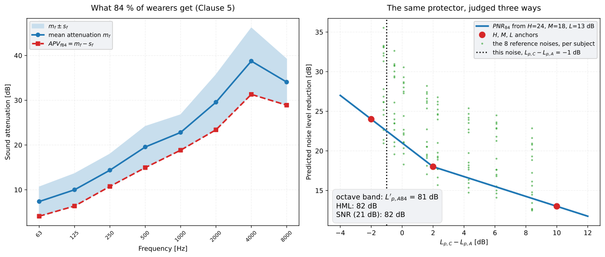

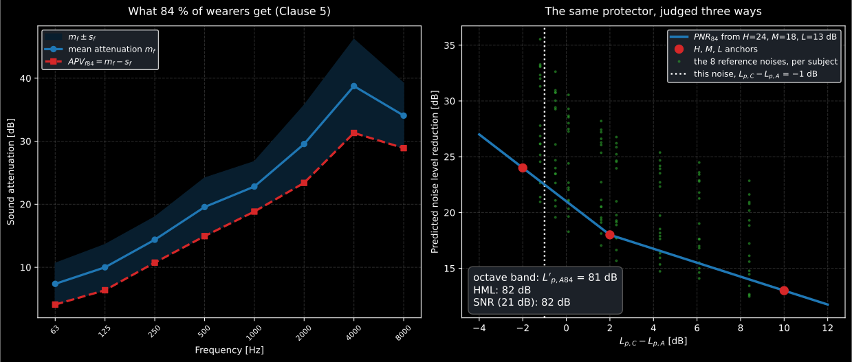
Left, the protector: the assumed protection value sits a full standard deviation below the mean, and the gap is widest where the spread is, at 4 kHz. Right, the method: the HML line and the eight reference noises it was fitted on, with the three methods’ answers for the same noise.

import matplotlib.pyplot as plt

# apv is the AssumedProtectionResult computed above. One line:
apv.plot()   # mean, its spread shaded, and the assumed protection on top
plt.show()

# The HML side, by hand.
hml = hearing.hml_rating(attenuation)
high, medium, low = hml.reported
left, right = np.array([-4.0, 2.0]), np.array([2.0, 12.0])
fig, ax = plt.subplots()
ax.plot(left, medium - (high - medium) / 4 * (left - 2), color="#1f77b4")
ax.plot(right, medium - (medium - low) / 8 * (right - 2), color="#1f77b4")
ax.plot([-2, 2, 10], [high, medium, low], "o", color="#d62728", label="H, M, L")
differences = np.asarray(hearing.HML_REFERENCE_C_MINUS_A)
ax.plot(np.repeat(differences, 16), hml.predicted_reduction.T.reshape(-1), ".",
        color="#2ca02c", alpha=0.5, label="reference noises")
ax.set(xlabel="LpC - LpA [dB]", ylabel="Predicted noise level reduction [dB]")
ax.legend()
plt.show()

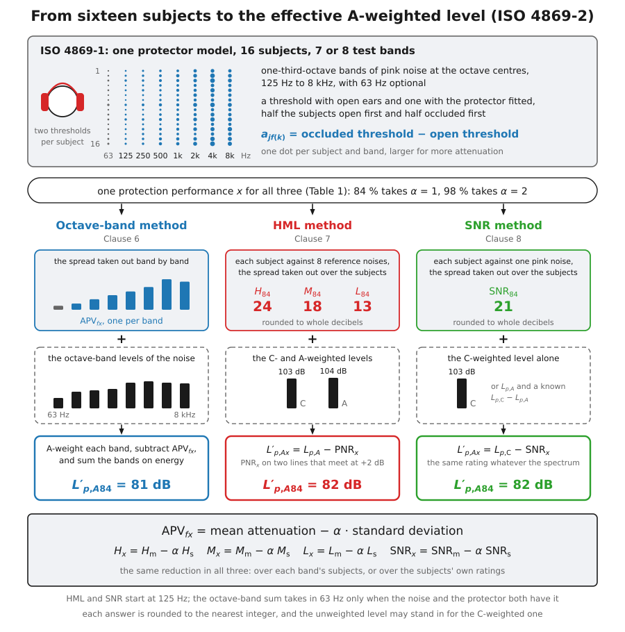
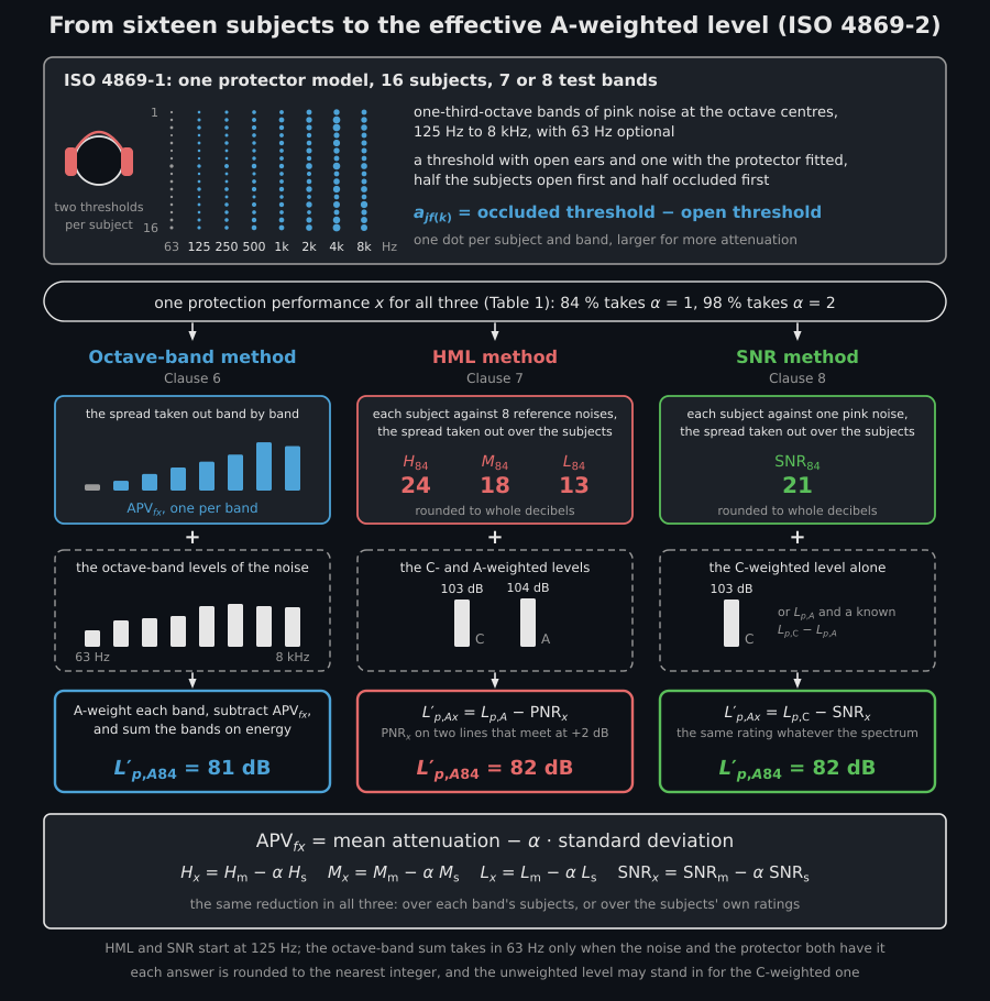
One protector model on sixteen subjects, reduced three ways and met with one noise. Only the octave-band method goes through the assumed protection value; HML and SNR rate each subject first and take the spread out over those ratings, and the three land within a decibel of each other.

The most faithful, and the only one that sees the shape of the noise: subtract the assumed protection value band by band from the A-weighted spectrum and sum what is left.

# Annex B's noise: octave-band levels of a machine hall, LpA = 104 dB.
noise = [75.0, 84.0, 86.0, 88.0, 97.0, 99.0, 97.0, 96.0]
octave = hearing.octave_band_protected_level(noise, apv)
print(round(octave.effective_level, 1))   # 81.4
print(octave.reported_level)              # 81
print(round(octave.noise_reduction, 1))   # 22.6

The summation runs over the eight octaves from 63 Hz, or over seven from 125 Hz when either the noise or the protector has no 63 Hz data. Clause 6 rounds the result to the nearest integer, which is what reported_level does; effective_level keeps the unrounded value.

Three numbers instead of a spectrum. $H$, $M$ and $L$ are the predicted noise level reduction this protector gives for reference noises whose $(L_{p,C}-L_{p,A})$ is $-2$, $+2$ and $+10$ dB, fitted across the eight reference spectra of Table 2. Applying them needs only the C- and A-weighted levels of the real noise:

hml = hearing.hml_rating(attenuation)
print(hml.reported)                       # (24, 18, 13)

by_hml = hearing.hml_protected_level(104.0, 103.0, hml)
print(round(by_hml.noise_reduction, 1))   # 22.5
print(by_hml.reported_level)              # 82

Both branches meet at $+2$ dB, which is where $M$ itself is defined, so the line has a corner and no step. The values that enter them are the rounded ones: Clause 7.2 rounds $H$, $M$ and $L$ to the nearest integer, which is what a protector is published with, so that is what the application consumes.

One number, against a pink noise, subtracted from the C-weighted level.

snr = hearing.snr_rating(attenuation)
print(snr.reported)                       # 21

by_snr = hearing.snr_protected_level(snr, l_p_c=103.0)
print(by_snr.reported_level)              # 82

# When only the A-weighted level was recorded, Formula (24) reassembles the
# C-weighted one from an estimate of the difference and lands in the same place.
print(hearing.snr_protected_level(snr, l_p_a=104.0, c_minus_a=-1.0).reported_level)  # 82

Clause 8.3 also allows the unweighted level in place of the C-weighted one, and Clause 7.3 says the same for HML. It reads high for noise with a lot of very low frequency content, so it is a fallback rather than an equivalent.

Because the reference noise is fixed, the rating says nothing about the shape of the noise it will meet, which is exactly what the HML method’s three values recover.

The three methods answer the same question and rarely agree exactly. On the worked example above the same protector in the same noise gives 81 dB, 82 dB and 82 dB, and the NOTE that closes the Introduction puts differences of 3 dB or less between comparable protectors below the resolution of the exercise. The ordering is not a ranking: the octave-band method uses more information and is the one to prefer when the spectrum is available, while HML and SNR exist precisely for when it is not.

The octave-band method starts at 63 Hz when both the noise and the protector have data there and at 125 Hz when either does not (Clause 6). The HML and SNR computations start at 125 Hz always, whatever is available at 63 Hz, which is why the reference spectra of Table 2 (Clause 7) and Table 3 (Clause 8) begin there.

One caution about the reference spectra: Annex C reprints Table 2 as its Table C.1 and the reprint disagrees with the original in two cells. Table 2 is the one that reproduces the annex’s own worked results, and it is the one this library carries; the discrepancy is registered in ERRATA.

An active noise reduction earmuff adds a cancellation circuit to a passive shell, and the circuit works mostly at low frequencies, where the shell is weakest. A threshold test cannot see it: ISO 4869-1 runs at levels far below those the circuit has anything to cancel. ISO 4869-6 therefore measures the two halves separately, on the same sixteen subjects, and adds them subject by subject. Its methods are meant for steady noise exposures and do not apply to noise with impulsive components (Clause 1):

• the passive attenuation is the ISO 4869-1 result with the circuit off, in octave bands;
• the active insertion loss (5.4.3) is the level at each ear with the circuit off minus the level with it on, measured with a microphone in the closed ear canal (ISO 11904-1) in one-third-octave bands of a broadband noise at 85 dB to 95 dB:

Annex A treats its uncertainty the way ISO 4869-1 treats the attenuation’s, over the sixteen values of the ear with the lower insertion loss, and prints an example, Table A.3:

# ISO 4869-6 Table A.3: the lower-ear active insertion loss of sixteen
# subjects at the octave frequencies 63 Hz to 8 kHz.
table_a3_anr = np.array([
    [18.4, 23.9, 21.6, 5.2, -4.5, -0.2, -1.3, -1.0], [19.4, 23.0, 21.7, 5.7, -6.4, -0.4, 0.8, -1.9],
    [19.7, 23.1, 20.8, 3.6, -4.2, -2.9, 0.2, -0.6], [19.8, 23.1, 18.7, 2.2, -4.9, -0.5, -0.2, 0.2],
    [20.5, 24.5, 20.2, 3.1, -4.4, -2.9, -1.4, 0.3], [18.8, 24.4, 20.8, 3.9, -4.3, -2.6, -0.4, -0.2],
    [21.7, 24.4, 22.2, 4.7, -5.2, -5.1, -1.5, -0.3], [20.5, 22.7, 24.3, 8.8, -8.8, -3.1, -4.8, -0.7],
    [22.9, 23.2, 20.7, 5.4, -6.5, -2.8, -0.5, -1.0], [21.9, 22.9, 23.1, 8.8, -8.4, -4.9, -2.6, -0.7],
    [23.7, 24.6, 20.8, 3.4, -6.4, -0.1, -0.3, -0.6], [22.0, 23.9, 20.3, 3.0, -4.2, -0.8, -1.0, 0.3],
    [23.2, 24.3, 20.9, 4.6, -5.6, -0.1, -0.5, -1.0], [21.5, 23.5, 23.3, 5.9, -5.2, -3.1, -3.6, -1.6],
    [24.3, 24.2, 22.5, 4.2, -6.3, -2.5, -0.9, -0.5], [23.8, 24.9, 20.7, 3.8, -4.8, -0.5, -0.3, 0.2],
])
insertion = hearing.active_insertion_loss(table_a3_anr)
print(np.round(insertion.mean_db, 1))                  # [21.4 23.8 21.4  4.8 -5.6 -2.  -1.1 -0.6]
print(np.round(insertion.expanded_uncertainty_db, 1))  # [0.9 0.4 0.7 0.9 0.7 0.8 0.7 0.3]

From 1 kHz up the circuit adds sound instead of removing it, up to 6 dB at 1 kHz, and the negative values are kept as they are. The mean and standard deviation rows of Table A.3 reproduce exactly, but its $u$ and $U_{95}$ rows are the formula applied to the rounded row above each ($1,4/4=0,35$ prints as 0,4), which puts six of its eight $U_{95}$ cells a tenth above the value A.1 and A.2 define. The library returns the defined value; the discrepancy is registered in ERRATA. Table A.2’s typical budget is hearing.ANR_WITHIN_LABORATORY_UNCERTAINTY, $U_{95}$ = 1.56 dB.

Clause 5.5 adds the two halves per subject. The passive attenuation is interpolated into one-third-octave bands and extended to 50 Hz and 10 kHz (a), only the ear with the lower active insertion loss is kept in each band (b), the two are added (c), each octave is the energetic average of its three one-third-octave bands (d), and the sixteen octave-band results go into the ISO 4869-2 methods at 84 % (e):

The standard sends the reader to a calculation workbook ISO publishes for the details, and that workbook interpolates linearly in hertz between the nominal centre frequencies, not on a logarithmic axis: 80 Hz lies 27 % of the way from 63 Hz to 125 Hz, not a third. The library follows the workbook and reproduces each step of 5.5 it stores: the ear with the lower value, the interpolation, the sums, Formula (1), and the mean, standard deviation and $AP{V}_{f84}$. The workbook rounds the interpolation, Formula (1), the mean and the standard deviation to 0.1 dB and leaves the rest as it comes; the library rounds nothing, which moves an octave-band total or an $AP{V}_{f84}$ by less than 0.1 dB.

# The REAT of the sixteen subjects, octave bands 63 Hz to 8 kHz.
reat_anr = np.array([
    [11.7, 15.7, 8.6, 10.7, 25.6, 22.7, 43.0, 38.0], [12.7, 20.3, 15.7, 13.4, 23.0, 24.3, 36.7, 42.0],
    [21.0, 22.7, 17.7, 18.0, 27.4, 31.0, 36.3, 45.0], [21.6, 22.0, 21.0, 13.4, 24.7, 30.3, 36.3, 42.3],
    [10.6, 10.0, 11.7, 16.0, 24.6, 23.4, 38.0, 42.4], [12.3, 13.3, 12.3, 17.6, 30.0, 22.6, 39.3, 43.3],
    [11.0, 10.0, 10.0, 13.6, 24.3, 25.4, 36.3, 37.4], [16.0, 12.0, 11.3, 13.0, 28.7, 25.7, 38.0, 35.0],
    [11.4, 11.6, 11.0, 13.7, 29.3, 24.3, 42.7, 37.6], [12.7, 12.0, 8.0, 9.0, 32.7, 25.6, 37.0, 41.0],
    [14.0, 10.3, 7.7, 15.0, 21.0, 22.7, 33.3, 33.0], [19.3, 18.3, 15.6, 16.3, 21.0, 26.4, 32.7, 31.0],
    [13.7, 15.4, 12.6, 13.4, 22.0, 19.0, 40.0, 33.3], [13.0, 15.3, 6.7, 12.0, 23.0, 28.7, 40.4, 38.0],
    [16.7, 21.6, 18.4, 18.0, 33.7, 37.7, 57.0, 50.6], [10.7, 15.0, 10.0, 11.7, 25.0, 22.0, 32.0, 38.7],
])
# Their lower-ear active insertion loss, 24 one-third octaves 50 Hz to 10 kHz.
ail_anr = np.array([
    [17.3, 18.4, 20.6, 23.3, 23.9, 24.8, 23.6, 21.6, 17.0, 12.1, 5.2, -0.7, -5.7, -4.5, -2.0, 0.1, -0.2, -6.5, -4.4, -1.3, -0.2, 0.2, -1.0, -0.1],
    [17.5, 19.4, 19.9, 21.7, 23.0, 23.9, 23.9, 21.7, 17.6, 12.8, 5.7, 0.8, -6.8, -6.4, -2.6, -1.2, -0.4, -1.6, -0.8, 0.8, -0.4, -1.3, -1.9, 0.7],
    [17.0, 19.7, 21.2, 22.0, 23.1, 24.6, 23.7, 20.8, 17.0, 11.6, 3.6, -2.0, -7.0, -4.2, -1.9, -0.6, -2.9, -6.2, -2.8, 0.2, 0.3, -1.0, -0.6, 0.6],
    [17.4, 19.8, 21.3, 22.4, 23.1, 22.3, 20.6, 18.7, 14.6, 9.7, 2.2, -2.6, -6.3, -4.9, -2.5, -1.4, -0.5, -2.9, -1.1, -0.2, 0.2, 0.1, 0.2, 1.1],
    [19.0, 20.5, 21.8, 23.1, 24.5, 24.5, 22.3, 20.2, 16.2, 10.6, 3.1, -1.5, -5.9, -4.4, -1.6, -0.8, -2.9, -7.7, -5.8, -1.4, 0.0, -0.6, 0.3, -0.7],
    [17.7, 18.8, 20.4, 23.0, 24.4, 25.3, 24.3, 20.8, 16.4, 10.6, 3.9, -1.7, -6.2, -4.3, -2.0, -1.2, -2.6, -5.1, -3.9, -0.4, 0.3, -0.1, -0.2, 0.3],
    [20.0, 21.7, 22.8, 23.2, 24.4, 24.1, 24.2, 22.2, 17.3, 12.5, 4.7, 0.2, -5.5, -5.2, -2.4, -1.5, -5.1, -8.7, -6.6, -1.5, -1.1, -1.7, -0.3, -0.4],
    [20.1, 20.5, 21.2, 21.4, 22.7, 24.7, 25.1, 24.3, 19.7, 15.5, 8.8, 5.4, -3.3, -8.8, -7.6, -4.1, -3.1, -6.2, -8.3, -4.8, -2.1, -0.6, -0.7, -1.9],
    [22.9, 22.9, 22.9, 22.9, 23.2, 24.0, 23.6, 20.7, 17.2, 11.7, 5.4, 0.1, -7.7, -6.5, -3.0, -1.9, -2.8, -3.9, -4.5, -0.5, 0.0, -0.7, -1.0, 1.1],
    [21.9, 21.9, 21.9, 21.9, 22.9, 24.3, 24.4, 23.1, 17.8, 14.3, 8.8, 5.3, -3.4, -8.4, -4.8, -2.7, -4.9, -5.0, -4.2, -2.6, -0.3, -0.4, -0.7, -0.4],
    [23.7, 23.7, 23.7, 23.7, 24.6, 24.3, 23.0, 20.8, 16.7, 11.1, 3.4, -2.2, -8.0, -6.4, -3.0, -1.7, -0.1, 0.0, -0.5, -0.3, -0.2, -1.8, -0.6, 0.0],
    [22.0, 22.0, 22.0, 22.0, 23.9, 24.1, 22.8, 20.3, 16.1, 11.1, 3.0, -1.8, -6.2, -4.2, -1.9, -0.1, -0.8, -6.0, -5.2, -1.0, -0.2, 0.1, 0.3, 0.7],
    [23.2, 23.2, 23.2, 23.2, 24.3, 23.9, 23.5, 20.9, 16.8, 11.8, 4.6, -1.2, -6.8, -5.6, -2.3, -1.2, -0.1, -1.5, -3.2, -0.5, 0.8, 0.1, -1.0, -0.3],
    [21.5, 21.5, 21.5, 21.5, 23.5, 24.6, 25.1, 23.3, 17.6, 13.4, 5.9, 1.6, -4.3, -5.2, -2.3, -1.2, -3.1, -7.3, -4.0, -3.6, 0.0, -1.3, -1.6, 0.6],
    [24.3, 24.3, 24.3, 24.3, 24.2, 24.6, 23.9, 22.5, 17.7, 12.4, 4.2, -0.2, -7.2, -6.3, -2.2, -1.0, -2.5, -6.9, -3.1, -0.9, 0.0, -0.1, -0.5, 0.6],
    [23.8, 23.8, 23.8, 23.8, 24.9, 24.2, 22.3, 20.7, 15.9, 10.9, 3.8, -0.4, -6.7, -4.8, -2.1, -0.7, -0.5, -6.3, -3.4, -0.3, 0.2, 0.1, 0.2, 1.3],
])

anr = hearing.anr_total_attenuation(reat_anr, ail_anr)
print(np.round(anr.assumed_protection.apv, 1))  # [31.6 34.5 29.1 16.9 15.2 19.9 27.8 33.5]
print(anr.hml.reported, anr.snr.reported)       # (21, 17, 19) 21

# The same earmuff with the circuit off, straight into ISO 4869-2:
print(hearing.hml_rating(reat_anr).reported, hearing.snr_rating(reat_anr).reported)
# (24, 17, 12) 20

The circuit buys seven decibels of $L$, the low-frequency value, and costs three of $H$: it adds sound from 1 kHz up. The single number moves by one decibel, which is why a protector for a low-frequency noise is better chosen by $L$, or by the octave-band method, than by its SNR.

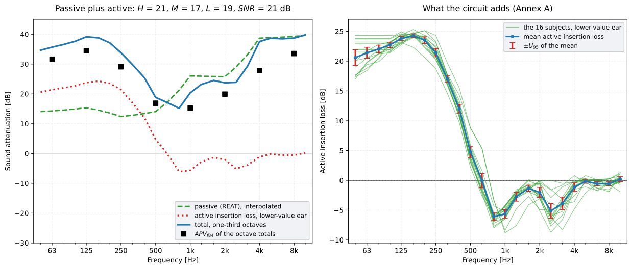
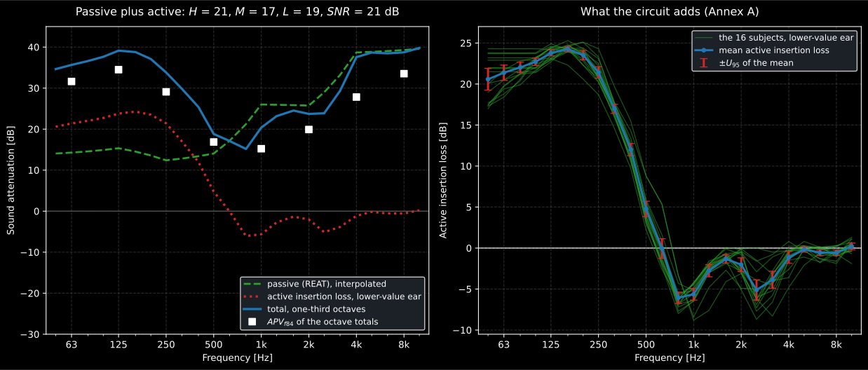
Left, ISO’s calculation example for 5.5: the circuit adds more than 20 dB where the passive shell is weakest, below 250 Hz, and takes a few decibels away from 1 kHz up. Right, the active insertion loss itself, the same data as Annex A: the spread between subjects is small, so its expanded uncertainty is too.

import matplotlib.pyplot as plt

anr.plot()  # passive, active and total, with the octave totals and the APV
plt.show()
# The workbook's lower-value-ear insertion loss in its 24 one-third octaves,
# of which Table A.3 is the octave-centre subset, with its expanded uncertainty.
hearing.active_insertion_loss(ail_anr).plot()
plt.show()

A cancellation circuit saturates, so its insertion loss only holds up to some external level. With red noise and the circuit on, the external A-weighted level rises in 5 dB steps from the insertion-loss level to at most 110 dB, and the level at each ear in the 125 Hz octave band shall rise by the same 5 dB, within ±1 dB. What is reported is the highest external level up to which that holds for every sample, subject and ear:

external = [90.0, 95.0, 100.0, 105.0, 110.0]
at_the_ears = [[60.0, 65.0, 70.0, 75.0, 80.0],   # one row per ear
               [61.0, 66.0, 71.0, 75.5, 78.0]]   # rises 2.5 dB on the last step
linearity = hearing.assess_anr_linearity(external, at_the_ears)
print(linearity.maximum_linear_level_db)  # 105.0
print(linearity.linear_to_110_db)         # False

The three one-third-octave levels at the ear can go in instead, as ear_third_octave_levels_db, and are summed into the octave on energy.

• Covered

  ISO 4869-1:2018’s attenuation of 4.6.2 and its statistics (4.6.3), the uncertainty of the mean of Annex A with the typical budgets of Tables A.2 and B.2, the significance test of Annex B (B.1.2, and the minimum difference of B.1.1 and B.2) and the sound-field conditions of 4.2.2 with Table 1, via hearing.real_ear_attenuation, hearing.assess_attenuation_difference, hearing.minimum_significant_difference, hearing.reat_expanded_uncertainty and hearing.check_reat_sound_field. Every derived cell of Tables A.2, A.3 and B.2, the criterion row and the verdict of Table B.1 and the four minimum differences are reproduced to the printed decimal in the test suite and in the conformance report. The difference row of Table B.1 agrees within 0.1 dB, because the standard prints the means of its second test rounded: at 8 kHz it comes out 3.94 dB against the printed 4,0.

• Covered

  ISO 4869-6:2019’s active insertion loss (5.4.1 and 5.4.3, from the MIRE levels of both ears or given directly), the choice of the ear with the lower value in 5.5 b), the uncertainty of its mean in Annex A with the typical budget of Table A.2, the total attenuation of 5.5 a) to e) with Formula (1), and the linear-operation check of 5.4.4, via hearing.active_insertion_loss, hearing.anr_total_attenuation and hearing.assess_anr_linearity. The mean and standard deviation of Table A.3 and its $u$ and $U_{95}$ rows as the table forms them are reproduced in the test suite and in the conformance report, and so is each step of 5.5 that ISO’s calculation workbook stores (rows 134-149, 182-197, 206-221, 230-245 and 247-249): the lower-ear rows exactly, the others within the rounding the workbook applies along the chain.

• Covered

  ISO 4869-2:2018’s assumed protection value (Clause 5, Formula (1), with all seven protection performances of Table 1), the octave-band method (Clause 6, Formula (2)), the HML method (Clause 7, Formulae (3) to (18), including the eight reference noises and the empirical weights of Table 2) and the SNR method (Clause 8, Formulae (19) to (24), against the pink noise of Table 3), via hearing.assumed_protection_value, hearing.octave_band_protected_level, hearing.hml_rating, hearing.hml_protected_level, hearing.snr_rating and hearing.snr_protected_level. Every printed number of the worked example that runs through Annexes A to D is reproduced in the test suite and in the conformance report.

• Not covered

  The threshold measurement itself is not simulated: ISO 4869-1’s subject selection and training (4.4), its fitting procedure (4.5), the test equipment (4.3), the reverberation time (4.2.3) and ambient noise (4.2.4, Table 2) of the test room and the application force of Clause 5 are laboratory requirements this library does not judge, and it starts from the thresholds or the attenuations they produced. The MIRE measurement of ISO 11904-1 behind the active insertion loss, the test signals of 5.3 and the oscillation check of 5.4.2 are likewise taken as given. ISO 4869-2’s Annex E uncertainty treatment of attenuation values and ratings is not implemented either. Nothing here models the difference between laboratory attenuation and what a protector achieves in the field, which is the subject of ISO/TR 4869-5 and is consistently large; a derating factor is a policy decision this library does not make for you.

References

Section titled “References”- International Organization for Standardization. (2018). Acoustics — Hearing protectors — Part 1: Subjective method for the measurement of sound attenuation (ISO 4869-1:2018). Where the per-subject attenuation values come from: the real-ear attenuation at threshold of 4.6, the uncertainty of its mean in Annex A, the significance test of Annex B and the sound-field qualification of 4.2.2 with its Table 1, validated against Tables A.2, A.3, B.1 and B.2 and the minimum differences of B.1.1 and B.2.
- International Organization for Standardization. (2018). Acoustics — Hearing protectors — Part 2: Estimation of effective A-weighted sound pressure levels when hearing protectors are worn (ISO 4869-2:2018). The implemented standard: the assumed protection value of Clause 5, the octave-band method of Clause 6, the HML method of Clause 7 and the SNR method of Clause 8, validated against the worked examples of Annexes A to D.
- International Organization for Standardization. (2019). Acoustics — Hearing protectors — Part 6: Determination of sound attenuation of active noise reduction earmuffs (ISO 4869-6:2019). The active insertion loss of 5.4, the ear with the lower value and its uncertainty (Annex A), the total attenuation of 5.5 and the linear-operation check of 5.4.4, validated against Tables A.2 and A.3 and against each step of 5.5 stored in the calculation workbook ISO publishes with it.