Source: https://jmrplens.github.io/phonometry/perception/psychoacoustics/loudness/ # Loudness Level metrics tell you how much *sound pressure* there is; loudness tells you how loud a listener actually *perceives* it. This page covers the reference method, loudness in sones by Zwicker (ISO 532-1), plus the equal-loudness contours of pure tones (ISO 226); the newer model families, Moore-Glasberg (ISO 532-2/-3) and the Sottek Hearing Model loudness (ECMA-418-2), are [Advanced loudness](https://jmrplens.github.io/phonometry/perception/psychoacoustics/advanced-loudness/). Sharpness, tonality and roughness live in [Sound Quality Metrics](https://jmrplens.github.io/phonometry/perception/psychoacoustics/sound-quality/); speech metrics in [Speech Transmission Index](https://jmrplens.github.io/phonometry/perception/speech/speech-transmission/) and [Speech Intelligibility Index](https://jmrplens.github.io/phonometry/perception/speech/speech-intelligibility/). ## Loudness in sones (ISO 532-1, Zwicker) Decibels compress perception: 10 dB more reads as *twice as loud*, and two sounds with the same dB(A) can differ audibly depending on how their energy spreads over the ear's **critical bands**. The Zwicker method models the hearing chain explicitly (outer/middle-ear transmission, critical-band analysis on the 24 Bark scale, level-dependent masking slopes) and outputs **loudness $N$ in sones**, a ratio scale: 4 sones is twice as loud as 2 sones. By definition a 1 kHz tone at 40 dB SPL is 1 sone, and every +10 phon doubles the sone value. 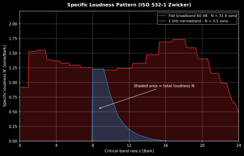The animation below shows that integration at work: as the band level of a 1 kHz narrowband sound steps up, the specific-loudness pattern $N'(z)$ grows along the Bark axis and the area under it is the total loudness in sones. [Watch the high-resolution video (WebM)](https://raw.githubusercontent.com/jmrplens/phonometry/main/.github/images/anim_specific_loudness.webm) ```python import numpy as np from phonometry import psychoacoustics # A raw recording plus its calibration so the guide runs standalone fs = 48000 x = 0.2 * np.sin(2 * np.pi * 1000 * np.arange(fs) / fs) # any recording (digital units) sens = 1.0 # calibration_factor to pascals levels_28 = np.full(28, 60.0) # 28 one-third-octave band levels (dB) # From a raw recording: calibration_factor scales digital units to Pa res = psychoacoustics.loudness_zwicker(x, fs, field="free", calibration_factor=sens) print(f"N = {res.loudness:.1f} sone ({res.loudness_level:.0f} phon)") # 13.1 sone (77 phon) # Time-varying signals: percentile loudness N5 is the reporting standard res = psychoacoustics.loudness_zwicker(x, fs) # stationary=False (default) print(f"{res.n5:.1f} {res.n10:.1f} {res.loudness:.1f}") # 13.1 13.1 13.1 — N5, N10, Nmax # From 28 one-third-octave band levels (25 Hz .. 12.5 kHz) res = psychoacoustics.loudness_zwicker_from_spectrum(levels_28, field="diffuse") res.plot() # N'(z) over the Bark scale — the specific-loudness pattern (needs matplotlib) ``` *Same band level, very different loudness: energy spread over many critical bands (red) sums to far more sones than the same level concentrated in one band (blue). The area under $N'(z)$ is the total loudness.*

Show the code for this figure

```python import matplotlib.pyplot as plt import numpy as np from phonometry import psychoacoustics levels_28 = np.full(28, 60.0) # 28 one-third-octave band levels (dB) # From 28 one-third-octave band levels (25 Hz .. 12.5 kHz) res = psychoacoustics.loudness_zwicker_from_spectrum(levels_28, field="diffuse") # One line — the specific-loudness pattern N'(z) straight from the result: res.plot() plt.show() # Or reproduce the figure by hand — two patterns of equal band level (60 dB), # energy spread over many critical bands vs concentrated in the 1 kHz band: narrow = psychoacoustics.loudness_zwicker_from_spectrum(np.r_[np.full(16, -60.0), 60.0, np.full(11, -60.0)]) broad = psychoacoustics.loudness_zwicker_from_spectrum(np.full(28, 60.0)) z = np.arange(1, narrow.specific.size + 1) * 0.1 # Bark axis fig, ax = plt.subplots() for r, color, label in [ (broad, "#ff7f0e", f"Broadband N = {broad.loudness:.1f} sone"), (narrow, "#1f77b4", f"1 kHz narrowband N = {narrow.loudness:.1f} sone"), ]: ax.fill_between(z, r.specific, color=color, alpha=0.3) ax.plot(z, r.specific, color=color, label=label) ax.set_xlabel("Critical-band rate z [Bark]") ax.set_ylabel("Specific loudness N' [sone/Bark]") ax.legend() plt.show() ```

The implementation is a clean-room port of the standard's **normative reference program** (Annex A.4): all twelve data tables are digit-exact and the full Annex B validation set runs in CI: the stationary test case reproduces the published value to every printed digit, and the tone-pulse $N(t)$ traces stay inside the standard's per-sample 5 % tolerance band. ### `loudness_zwicker()` parameters | Parameter | Type | Units | Range / default | Notes | | :--- | :--- | :--- | :--- | :--- | | `x` | 1D array | Pa (after calibration) | ≥ 8 ms at 48 kHz | Resampled internally to 48 kHz if needed | | `fs` | int | Hz | > 0 | | | `field` | str | — | `'free'` (default) / `'diffuse'` | Sound-field correction (Table A.5) | | `stationary` | bool | — | default `False` | `True`: single $N$ from the averaged spectrum | | `calibration_factor` | float | Pa per digital unit | default `1.0` | From `sensitivity()` | Returns a `ZwickerLoudness` dataclass: `loudness` ($N$, sones), `loudness_level` (phon), `specific` ($N'(z)$, 240 bins of 0.1 Bark), and for time-varying runs `n5`, `n10`, `time`, `loudness_vs_time` (500 Hz trace). ### ISO 532-1 report (`.report()`) `ZwickerLoudness.report(path)` renders a one-page PDF fiche laid out like an accredited loudness report: a standard-basis line, an optional metadata header block, a compact metrics table (total loudness $N$, loudness level $L_N$, and the $N_5$/$N_{10}$ percentiles for a time-varying result) beside the specific-loudness pattern $N'(z)$ (the result's own `.plot()`), the boxed $N = X\ \text{sone}$ ($L_N = Y\ \text{phon}$) single number, an optional verdict row and a footer with the fixed disclaimer. It uses the same `ReportMetadata` container (documented under [Insulation ratings](https://jmrplens.github.io/phonometry/buildings/insulation/insulation-ratings/#report-metadata-reportmetadata)) and rendering engine as the ISO 717 insulation fiche; a supplied `requirement` is read as the maximum permitted loudness in sone (a lower loudness passes). Rendering needs reportlab and, for the figure the fiche embeds, matplotlib (`pip install "phonometry[report,plot]"`); only `engine="reportlab"` is supported. The fiche renders in English by default; pass `language="es"` for a Spanish fiche (translated fixed strings and a comma decimal separator), e.g. `res.report("loudness_fiche_es.pdf", language="es")`. ```python from phonometry import psychoacoustics, ReportMetadata res = psychoacoustics.loudness_zwicker_from_spectrum(levels_28, field="free") res.report( "loudness_fiche.pdf", metadata=ReportMetadata( specimen="Household appliance, steady operating noise", measurement_standard="ISO 532-1 method 1", laboratory="Phonometry Reference Laboratory", requirement=12.0, # maximum permitted loudness (sone) ), ) # N (sone) and LN (phon) ``` The example fiche, regenerated with `make reports`, is kept rendered in the repository. 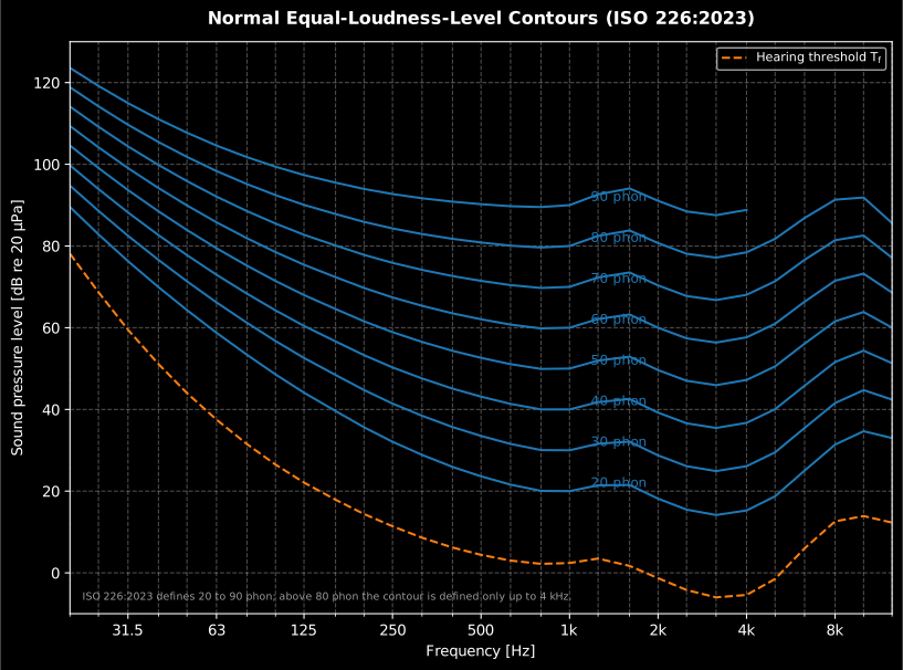Click the preview to open the PDF: [](https://raw.githubusercontent.com/jmrplens/phonometry/main/.github/reports/iso532_loudness_example.pdf) *Zwicker loudness fiche (`ZwickerLoudness.report`), N in sone with LN in phon.* ## Loudness level of pure tones (ISO 226:2023) The normal equal-loudness-level contours relate the SPL of a pure tone to its perceived *loudness level* in phons (the SPL of an equally loud 1 kHz tone). `equal_loudness_contour(phon)` evaluates ISO 226:2023 Formula (1) at the 29 preferred third-octave frequencies of Table 1, `loudness_level(spl, frequency)` is the exact inverse (Formula 2), and `hearing_threshold()` returns the threshold-of-hearing column. `equal_loudness_contours(phons)` bundles a whole family of contours with the threshold into a plottable `EqualLoudnessContours` result: ```python from phonometry import psychoacoustics freqs, spl = psychoacoustics.equal_loudness_contour(40.0) # the classic 40-phon contour phon = psychoacoustics.loudness_level(73.0, 63.0) # 73 dB @ 63 Hz -> 40 phon # The whole family (20-90 phon by default) plus the hearing threshold: res = psychoacoustics.equal_loudness_contours() res.plot() # the iconic ISO 226 chart (needs matplotlib) ``` ISO 226:2023 defines the contours from 20 to 90 phon; above 80 phon the formula is valid only up to 4 kHz, so the 90 phon contour stops there and no higher contours are defined.

Show the code for this figure

```python import matplotlib.pyplot as plt from phonometry import psychoacoustics # One line — the contour family straight from the result: res = psychoacoustics.equal_loudness_contours() res.plot() plt.show() # Or reproduce the figure by hand — ISO 226:2023 Formula (1) at the 29 # preferred frequencies of Table 1, one contour per loudness level: fig, ax = plt.subplots() for phon in [20, 40, 60, 80, 90]: freqs, spl = psychoacoustics.equal_loudness_contour(float(phon)) ax.semilogx(freqs, spl, color="C0") ax.annotate(f"{phon} phon", xy=(1000, phon + 1), fontsize=9) ft, tf = psychoacoustics.hearing_threshold() ax.semilogx(ft, tf, "--", color="C1", label="Hearing threshold $T_f$") ax.set(xlabel="Frequency [Hz]", ylabel="Sound pressure level [dB re 20 µPa]") ax.grid(True, which="both", alpha=0.3) ax.legend() plt.show() ```

Validity per clause 4.1: 20-90 phon (80 phon above 4 kHz); the implementation is verified against the Annex B tables in CI. The standard defines no interpolation between the 29 tabulated frequencies, so `loudness_level()` expects one of the Table 1 frequencies and rejects anything else. Note this is the loudness of *pure tones*; the loudness of arbitrary signals in sones is what the ISO 532 models compute, the Zwicker method above and the newer families of [Advanced loudness](https://jmrplens.github.io/phonometry/perception/psychoacoustics/advanced-loudness/). Zwicker is the reference model, not the only one. The **Moore-Glasberg** loudness of ISO 532-2, its time-varying ISO 532-3 extension and the **Sottek Hearing Model** loudness of ECMA-418-2, together with the model-choice table that says when to prefer each, are [Advanced loudness](https://jmrplens.github.io/phonometry/perception/psychoacoustics/advanced-loudness/). ## Quick answers ### What is the difference between loudness in sones and loudness level in phons? Loudness $N$ in sones (ISO 532-1) is a ratio scale of perceived loudness: 4 sones is twice as loud as 2 sones, and by definition a 1 kHz tone at 40 dB SPL is 1 sone. Loudness level in phons (ISO 226) is the SPL of an equally loud 1 kHz pure tone, and every +10 phon doubles the sone value. ### Over what range are the ISO 226:2023 equal-loudness contours valid? ISO 226:2023 clause 4.1 defines the normal equal-loudness-level contours from 20 to 90 phon, evaluated at the 29 preferred third-octave frequencies of Table 1; above 80 phon the formula is valid only up to 4 kHz, so the 90 phon contour stops there and no higher contours are defined. The contours describe pure tones, not arbitrary signals. ## References - Fastl, H., & Zwicker, E. (2007). *Psychoacoustics: Facts and models* (3rd ed.). Springer. [doi:10.1007/978-3-540-68888-4](https://doi.org/10.1007/978-3-540-68888-4). The critical-band and masking psychoacoustics behind the Zwicker model. - Fletcher, H., & Munson, W. A. (1933). Loudness, its definition, measurement and calculation. *The Journal of the Acoustical Society of America*, 5(2), 82-108. [doi:10.1121/1.1915637](https://doi.org/10.1121/1.1915637). The original equal-loudness measurements behind the loudness-level concept of the pure-tone section. - International Organization for Standardization. (2023). *Acoustics — Normal equal-loudness-level contours* (ISO 226:2023). [iso.org catalogue](https://www.iso.org/standard/83117.html). The contour model and Table 1 parameters behind the pure-tone loudness levels. ## Standards ISO 532-1:2017, *Acoustics — Methods for calculating loudness — Part 1: Zwicker method* — stationary and time-varying loudness in sones from the normative Annex A.4 reference program, with the N5/N10 percentile loudness, validated against the Annex B set. ISO 226:2023, *Acoustics — Normal equal-loudness-level contours* — the contours (Formula 1), the loudness level of pure tones (Formula 2) and the hearing threshold. ## See also - [Advanced loudness (ISO 532-2/-3, ECMA-418-2)](https://jmrplens.github.io/phonometry/perception/psychoacoustics/advanced-loudness/): the Moore-Glasberg and Sottek loudness models and the model-choice table. - [Sound Quality Metrics](https://jmrplens.github.io/phonometry/perception/psychoacoustics/sound-quality/): sharpness, tonality and roughness, the other half of the sound-quality story. - [Psychoacoustic annoyance and fluctuation strength](https://jmrplens.github.io/phonometry/perception/psychoacoustics/psychoacoustic-annoyance/): the Zwicker and Fastl model that consumes the percentile loudness $N_5$. - [Theory](https://jmrplens.github.io/phonometry/reference/theory/perception/): the equations behind the loudness models. - API reference: [`psychoacoustics.loudness.zwicker`](https://jmrplens.github.io/phonometry/reference/api/psychoacoustics/zwicker/) and [`psychoacoustics.loudness.contours`](https://jmrplens.github.io/phonometry/reference/api/psychoacoustics/contours/).