Calibration and dBFS
Standards: IEC 60942AES17IEC 61672Key references: Bies et al. 2017
Every level this library reports is only as trustworthy as the one number this page produces: the sensitivity factor that converts digital units into pascals. The page covers both reference frames a recording can be analyzed in: physical dB SPL, obtained by calibrating the chain against an IEC 60942 acoustic calibrator, and digital dBFS, levels relative to full scale with no physical claim attached.
Choosing between them is a question about your measurement chain, not about preference. Work in dB SPL whenever the result faces a physical criterion (a noise limit, an exposure threshold, any acoustics standard); that requires a calibrator recording made through the same, untouched chain as the measurement. Work in dBFS when the signal never had a calibrated analog front end (loudness normalization, codec and interface tests, file-only analysis) or when no calibration tone exists, in which case absolute SPL statements are simply out of reach.
The workflow around the factor matters as much as the formula: derive it before and re-check it after each session, verify meter and calibrator periodically in the laboratory (IEC 61672-3 and IEC 60942; Bies, Hansen & Howard 2017, §3.4), and treat the pre/post difference as your drift bound. The field, laboratory and drift section below turns that into concrete rules, and the Build a sound level meter walkthrough starts from exactly this step before any level is computed.
Why calibrate? The theory
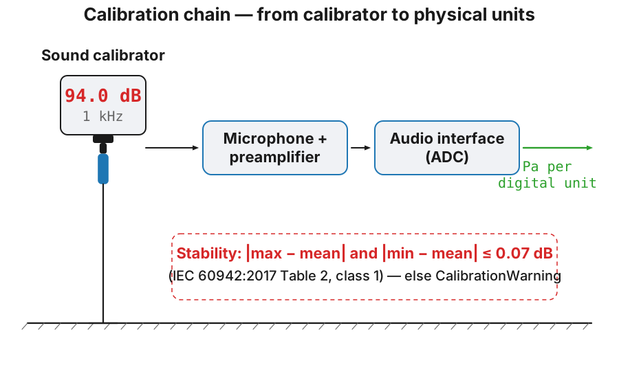
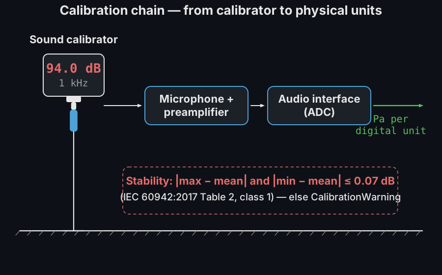
Section titled “Why calibrate? The theory”A digital recording only knows numbers: a full-scale sine wave is ±1.0 regardless of whether it was a whisper or a jet engine. To report physical sound pressure levels the chain microphone → preamplifier → ADC must be characterised by a single number, the sensitivity factor , that converts digital units into pascals:
where is the calibrator’s level (typically 94 dB, i.e. 1 Pa),
and is the RMS of
the recorded calibration tone in digital units. sensitivity() is
exactly that equation. The factor is valid as long as nothing in the chain
changes: touch the gain knob and you must recalibrate.
Calibrating a recording, end to end
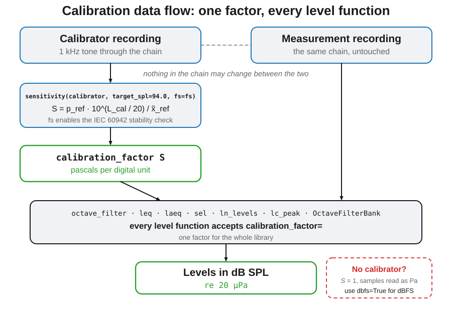
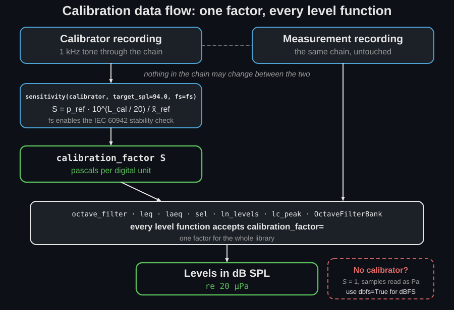
Section titled “Calibrating a recording, end to end”The three steps below are the whole physical-SPL workflow: a calibrator take,
one call to sensitivity(), and the factor handed to a level function. Both
recordings must come from the same chain with nothing touched in between. The
same factor works across the whole library: octave_filter and
OctaveFilterBank take it inside LevelCalibration(factor=...), and leq,
laeq and ln_levels as calibration_factor=.
import numpy as npfrom phonometry import filters, metrology
# 1. Record your 94 dB calibrator signal (1 kHz, 1 Pa RMS = 94 dB SPL)fs = 48000# calibrator_recording: your recorded 1 kHz calibrator tone (1 Pa RMS = 94 dB SPL).#   Synthesized here so the guide runs; in a real measurement, record your calibrator.#   Five seconds, as the coupling procedure below asks for.calibrator_recording = np.sqrt(2) * np.sin(2 * np.pi * 1000 * np.arange(5 * fs) / fs)# recording: the mic capture you want to calibrate, same input chain (Pa after calibration).#   Synthesized here; in a real measurement this is your recorded signal.recording = 0.2 * np.sin(2 * np.pi * 1000 * np.arange(fs) / fs)
# 2. Calculate the sensitivity factorcalibration_factor = metrology.sensitivity(calibrator_recording, target_spl=94.0, fs=fs)
# 3. Apply calibration to your measurementsfiltered = filters.octave_filter(    recording, fs,    calibration=filters.LevelCalibration(factor=calibration_factor))spl, freq = filtered.levels, filtered.frequencies# spl is now in dB SPL re 20 µPaprint(f"S = {calibration_factor:.3f} Pa per digital unit")   # 1.002print(f"1 kHz band: {spl[freq.index(1000.0)]:.1f} dB SPL")   # 77.0
Both numbers are worth reading rather than skipping. The synthetic calibrator take has an RMS of exactly 1.0 digital unit, so Pa per digital unit: one digital unit is one pascal, which is what a chain whose full scale sits just above the calibrator level looks like. The measurement record has amplitude 0.2, hence an RMS of 0.141 digital units, hence 0.142 Pa, hence dB SPL: the 1 kHz band the snippet prints.
That gives the sanity rule for every later session. is the pascal-per-unit
scale of the chain, so (the calibrator level minus the
RMS level of the calibrator take in dBFS) is the sound pressure level that
would drive the converter to a digital RMS of 1.0. If that number is not within
a few decibels of the loudest level the chain was set up for, something is wrong
with the take: a clipped or half-scale recording, a target_spl left at 94.0 for
a 114 dB calibrator, or a gain change between the two recordings. A factor wrong
by exactly 20 dB is the usual outcome of the second mistake, and no later step
will reveal it.
Coupling the calibrator
Section titled “Coupling the calibrator”The snippet is three lines; the step it hides is the one that goes wrong. The specified level of a sound calibrator is the level at the diaphragm of the inserted microphone (IEC 60942:2017, 5.3.1.2), so the mechanical assembly is part of the measurement, not a preliminary to it. Six steps:
- Set the gain for the loudest level you expect, and lock it. is valid only while the chain stays exactly as calibrated, and a gain knob moved after the check shifts every level by an amount nothing downstream can detect.
- Disable every automatic process on the interface (gain riding, limiting, noise suppression, “voice” enhancement) and record at 24 bit. Any of them makes the chain non-linear, and the calibrator take is the one signal on which that is invisible, because it is a single steady tone.
- Take the windscreen off and fit the adaptor supplied with the calibrator. An adaptor is an integral part of the sound calibrator (5.1.1), and where the manual gives adaptor design data it also gives the insertion distance and the minimum microphone diameter at which sealing occurs (6.3 u). Check that your microphone model and configuration (with or without the protective grid) is in the manual’s list (6.3 a): the specified level holds for the models and configurations stated there (5.3.1.3), and the manual states how much the level moves with the effective load volume of the inserted microphone (6.3 k), the air volume bounded by the reference plane, the diaphragm and the capsule wall (3.13).
- Insert the capsule fully to the reference plane (the plane of contact between microphone and calibrator, 3.12), hold the assembly still and let it settle. The manual states two settling times: the calibrator’s own, which may not exceed 30 s (5.1.10), and the time the microphone-and-calibrator combination needs after they are coupled (6.3 e).
- Do the check away from the running source. The cavity is not a sound
isolator. IEC 60942 makes this quantitative for its own tests: with the
microphone coupled and the calibrator switched off, the level the microphone
reads must be at least 30 dB below the level being measured for periodic
testing (B.4.2), and 40 dB below for pattern evaluation (A.5.3). For a 94 dB
calibrator that is a background below 64 dB at the capsule (a number you can
record and check in ten seconds, and the one that decides whether
narrowband=Trueis optional (see the figure below). - Record 5 to 10 s of settled tone, trim the handling noise at both ends,
and pass the rest to
sensitivity(ref, fs=fs). The standard measures the generated level as an average over 20 s to 25 s (A.5.5.1) and the short-term fluctuation over 60 s sampled at least 30 times (5.3.3); a few settled seconds is enough for the RMS to converge, and the stability check below is what tells you the tone really was settled.
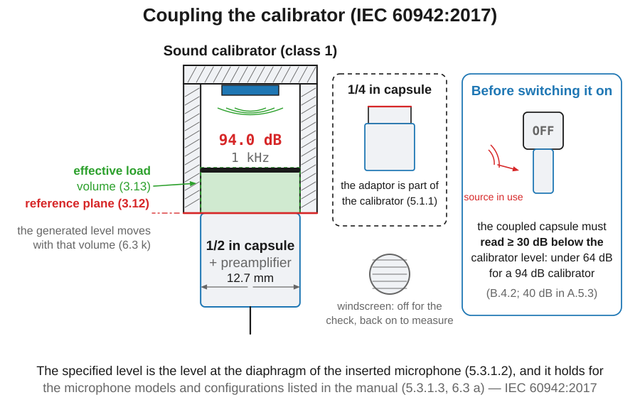
Pressure field in the cavity, free field in the measurement. The coupler drives the diaphragm with a pressure excitation: the cavity is far smaller than a wavelength, so the sound pressure is uniform over it and no diffraction around the capsule takes place. The microphone you are calibrating is normally rated for a free field, where its own body and the grid raise the response at high frequency. The two ratings differ by tenths of a decibel below about 2 kHz and by several decibels near 10 kHz, which is why IEC 60942 confines the principal frequency of a sound calibrator to the 160 Hz to 1250 Hz range (5.4.1.1): there the pressure and free-field sensitivities of a measurement capsule coincide closely enough that no correction is applied. It also means is a single-frequency anchor. The shape of the chain’s response away from the calibrator frequency comes from the microphone’s own free-field data, not from this check; the three sensitivities and where each applies are laid out in Microphones. Put the windscreen back on before measuring, and remember it has its own insertion loss of a few tenths of a decibel at high frequency, which the calibration did not see.
Calibrator assumptions (IEC 60942)
Section titled “Calibrator assumptions (IEC 60942)”sensitivity assumes the reference recording comes from an acoustic
calibrator as specified by IEC 60942 (classes LS, 1 and 2):
- The default
target_spl=94.0matches the common 94 dB @ 1 kHz calibrator output. Clause 5.3.1.3 requires the principal level to be at least 90 dB re 20 µPa when the calibrator is applied to the microphone models and configurations specified in its instruction manual; 94 dB and 114 dB are the usual choices, and the principal frequency must lie between 160 Hz and 1.25 kHz (5.4.1.1). - The resulting sensitivity inherits the calibrator’s own level tolerance, and that number takes one step to obtain. IEC 60942:2017 deliberately does not print tolerance limits: Table 2 gives the acceptance limit on the generated level (0.25 dB for a class 1 calibrator from 160 Hz to 1.25 kHz, 0.40 dB for class 2, 0.10 dB for class LS) and Table A.1 the maximum-permitted uncertainty of the laboratory measurement that demonstrates it (0.15 dB for class 1 over the same range); Annex D, Figure D.1 places the tolerance limit at their sum. ±0.4 dB is therefore the class 1 figure to carry into an uncertainty budget at 1 kHz, and it is a tolerance, not a measured error. Add the RMS estimation error of your own recording on top of it.
- IEC 60942 measures the generated level as an average over 20 s to 25 s (A.5.5.1): record a few seconds of stable tone (excluding handling noise at the start/end) for the RMS estimate to converge.
- Environmental corrections, and which calibrators need them. The generated level is specified at the reference conditions of Clause 4: 23 °C, 101.325 kPa and 50 % relative humidity. Table 2 still applies without any correction over a band around them (97 kPa to 105 kPa, 20 °C to 26 °C, 40 % to 65 % RH, clause 5.3.2), and outside that band a calibrator must stay inside the wider limits of Tables 5 and 6 over its whole operating range, which for class 1 is 65 kPa to 108 kPa, −10 °C to +50 °C and 25 % to 90 % RH (5.5). Only pistonphones that need a static-pressure correction to meet their class carry the letter M in their designation (class LS/M, class 1/M, 5.1.5 and Table 1); they are supplied with a barometer, or their manual specifies one (5.1.8), and the manual states the correction and its uncertainty (6.3 i, 6.3 m). A pistonphone generates a fixed volume displacement, so its output follows the ambient static pressure (of order a tenth of a decibel for ordinary weather and around −1 dB at 1000 m above sea level). Every other calibrator, by 5.1.7, must meet its class with no environmental correction at all. When a correction is required, apply it to the target level and not to the results:
p_correction_db = 0.0 # from the calibrator manual and the barometer readingcal_corrected = metrology.sensitivity( calibrator_recording, target_spl=94.0 + p_correction_db, fs=fs)The correction enters directly, so it moves every level of the session by the same amount.
Automatic stability validation
Section titled “Automatic stability validation”When you pass the sample rate (and validate=True, the default),
sensitivity(ref, fs=fs) checks the recording the way
IEC 60942:2017 checks the calibrator itself (5.3.3): the short-term level
fluctuation, the absolute difference between each of the maximum and minimum
F-time-weighted levels and the mean level, must not exceed the Table 2 limit
for the calibrator’s class and nominal frequency, read from the published
metrology.FLUCTUATION_ACCEPTANCE_LIMITS_DB. For class 1, the default,
Table 2 gives three disjoint rows, and they must not be read as overlapping
ranges:
| Nominal frequency | Class 1 limit | |
|---|---|---|
| 160 Hz to 16 kHz | 0.07 dB | the strict row, and the one a 1 kHz calibrator is judged on |
| above 63 Hz to below 160 Hz | 0.10 dB | |
| 31.5 Hz to 63 Hz | 0.20 dB | where the F time weighting itself ripples on the tone |
Table 2 spans 31.5 Hz to 16 kHz and specifies nothing outside it, so a
frequency below 31.5 Hz or above 16 kHz falls back to the strict 0.07 dB
rather than to the relaxed low-frequency rows. Pass frequency= to select the
right row for non-1 kHz calibrators, and calibrator_class= to select the
column: a class LS calibrator is held to 0.03 dB and a class 2 one to 0.15 dB,
both specified from 160 Hz to 1.25 kHz only, and outside that span the
strictest figure of the class’s own column applies, as it does for class 1.
A CalibrationWarning flags badly coupled microphones or handling
noise before they silently corrupt every calibrated level. The recording must
be at least 2 s long (1 s for the F-integrator to settle plus 1 s of settled
envelope); shorter recordings get a warning instead of an unreliable verdict.
Without fs the check is skipped. Override the limit with
max_fluctuation_db or disable with validate=False.
The check catches exactly what ruins field calibrations (a loose coupler, wind, handling noise):
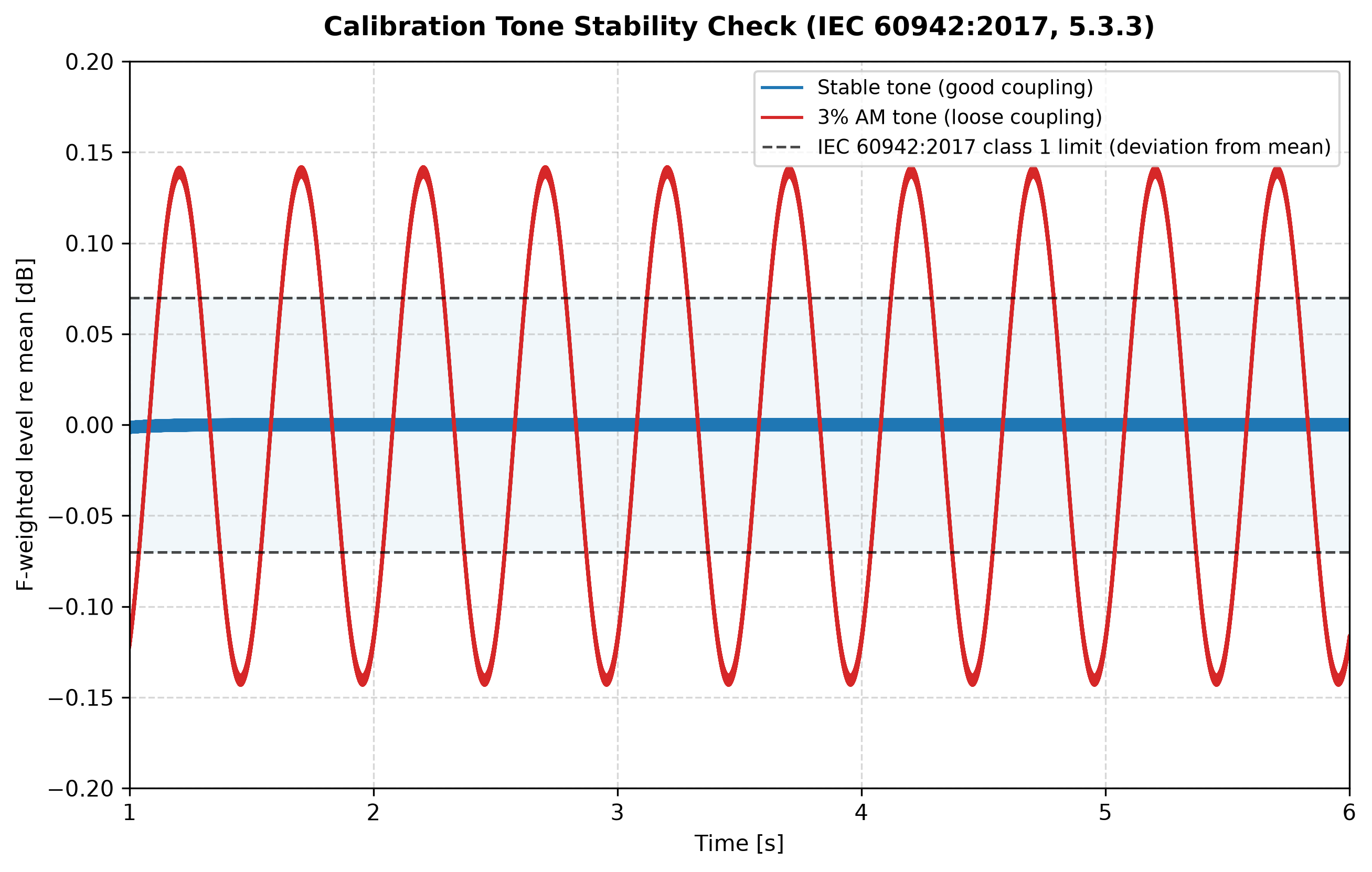
The check is a decision, and the figure shows how far from marginal it is. The stable tone wanders between +0.003 and −0.004 dB about its mean, a twentieth of the 0.07 dB Table 2 class 1 limit. Three per cent of amplitude modulation (a coupler that is not quite seated, a hand on the microphone) takes it to +0.142 and −0.143 dB, twice the limit, while sounding identical and reading the same mean level. The mean is what the sensitivity uses; only the fluctuation says whether it can be trusted.
Show the code for this figure
import matplotlib.pyplot as pltimport numpy as npfrom phonometry import filters
fs = 48000t = np.arange(int(fs * 6.0)) / fsstable = 0.5 * np.sin(2 * np.pi * 1000 * t)# 3 % amplitude modulation at 2 Hz: ~0.14 dB of wobble, clearly overunstable = stable * (1 + 0.03 * np.sin(2 * np.pi * 2.0 * t))
plt.figure(figsize=(9, 5))skip = fs                     # discard the F-integrator attack (~8 tau)for x, label in ((stable, "Stable tone (good coupling)"),                 (unstable, "3% AM tone (loose coupling)")):    env = filters.time_weighting(x, fs, mode="fast")[skip:]    level = 10 * np.log10(np.maximum(env, np.finfo(float).eps))    plt.plot(t[skip:], level - level.mean(), label=label)for lim in (0.07, -0.07):    plt.axhline(lim, linestyle="--", color="gray")plt.xlabel("Time [s]")plt.ylabel("F-weighted level re mean [dB]")plt.legend()plt.show()
Broadband noise in the take, and what it costs
Section titled “Broadband noise in the take, and what it costs”The RMS of the calibrator recording is the denominator of , so anything in
the take that is not the tone inflates it and shrinks the factor; and every
level derived from that factor then reads low, by
with SNR the tone-to-noise power ratio in the
recording. Passing narrowband=True replaces the full-band RMS with a coherent
Goertzel detector locked to the tone, which rejects the incoherent part:
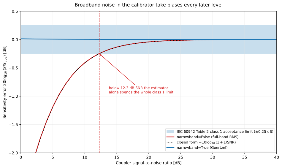
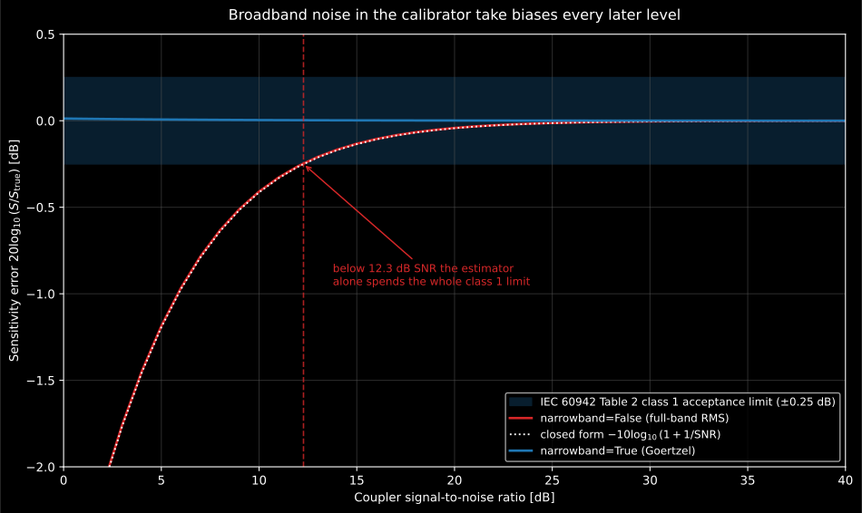
Sensitivity error against the signal-to-noise ratio of the calibrator take,
measured by calling sensitivity() on a 1 kHz tone plus broadband noise. The
full-band RMS estimator lands exactly on the closed form; it costs 0.41 dB at
10 dB SNR, 0.05 dB at 20 dB and spends the whole class 1 acceptance limit of
0.25 dB below 12.3 dB SNR. The Goertzel estimator stays inside 0.02 dB
everywhere. The 30 dB background margin the coupling procedure asks for
(B.4.2) therefore puts the plain RMS estimator at 0.004 dB, which is why
narrowband=False is a sane default and narrowband=True is the repair for a
take you could not make quiet enough.
Show the code for this figure
import matplotlib.pyplot as pltimport numpy as np
# metrology comes from the first snippet on this page.fs = 48000t = np.arange(int(fs * 6.0)) / fstone = np.sqrt(2) * np.sin(2 * np.pi * 1000 * t)     # 1 Pa RMS on 1.0 digitals_true = 2e-5 * 10 ** (94 / 20)noise = np.random.default_rng(7).standard_normal(t.size)noise /= np.sqrt(np.mean(noise ** 2))
snr_db = np.arange(0.0, 40.5, 1.0)rms, goertzel = [], []for snr in snr_db:    x = tone + noise * 10 ** (-snr / 20)    # validate=False: the noisy takes deliberately fail the stability check,    # which is a second, independent reason not to accept them.    rms.append(        20 * np.log10(metrology.sensitivity(x, fs=fs, validate=False) / s_true))    goertzel.append(20 * np.log10(        metrology.sensitivity(x, fs=fs, narrowband=True, validate=False) / s_true))
plt.figure(figsize=(9, 5))plt.axhspan(-0.25, 0.25, alpha=0.15)plt.plot(snr_db, rms, label="narrowband=False")plt.plot(snr_db, -10 * np.log10(1 + 10 ** (-snr_db / 10)), "k:",         label="closed form")plt.plot(snr_db, goertzel, label="narrowband=True")plt.xlabel("Coupler signal-to-noise ratio [dB]")plt.ylabel("Sensitivity error [dB]")plt.legend()plt.show()
sensitivity() parameters
Section titled “sensitivity() parameters”| Parameter | Type / shape | Units | Range / default | Notes |
|---|---|---|---|---|
ref_signal | 1D/2D array | digital units | non-empty, non-silent | Recording of the calibration tone only (trim handling noise) |
target_spl | float | dB re 20 µPa | default 94.0 | The calibrator’s nominal level (114 dB calibrators: pass 114.0) |
reference_pressure_pa | float | Pa | default 2e-5 | Reference pressure ; rarely changed |
fs | int, optional | Hz | > 0; default None | Required for the stability validation; omit to skip it |
validate | bool | — | default True | Emit CalibrationWarning on unstable/short recordings; needs fs, and does nothing without it |
max_fluctuation_db | float, optional | dB | default None → Table 2, by class and frequency | Explicit override of the stability limit |
frequency | float | Hz | default 1000.0 | Calibrator’s nominal frequency; selects the IEC 60942 Table 2 row |
calibrator_class | str | — | 'LS', 'LS/M', '1', '1/M', '2'; default '1' | Calibrator’s class designation (Table 1); selects the Table 2 column |
narrowband | bool | — | default False | Estimate the tone with a coherent Goertzel detector near frequency (needs fs) instead of full-band RMS; rejects broadband hum/noise that otherwise inflates the RMS and shrinks every later level (−0.41 dB at 10 dB SNR, −0.04 dB at 20 dB; see the figure above). Enable for noisy coupler recordings |
Returns the sensitivity factor (float) to pass as calibration_factor= to
leq, laeq, ln_levels, lc_peak, sel and the dose functions, and as
calibration=LevelCalibration(factor=...) to octave_filter.
What the factor also tells you: the measurable range
Section titled “What the factor also tells you: the measurable range”is not only a conversion, it is the chain’s scale, and both ends of the measurable range fall straight out of it.
The ceiling. A signal whose digital RMS reaches 1.0 corresponds to dB, which is also the calibrator level minus the dBFS level of the calibrator take. A full-scale sine has an RMS of , so it reads 3.01 dB lower, . That is the highest sine level the converter can carry without clipping; compare it against the microphone’s own overload sound pressure level, which is a capsule-and-preamplifier property and not a converter one (see Microphones), and keep the smaller of the two at least 10 dB above the loudest event you expect. A clipped event does not announce itself: it reads low, and plausibly so.
The floor. Record 30 s with the capsule in a quiet enclosure (the closed calibrator cavity with the drive switched off does nicely, which is the same take the coupling step already asks for) and run it through the same factor. That level is the chain’s inherent noise, microphone plus preamplifier plus converter. A measured level within 3 dB of it is not a measurement of the source; one within 10 dB needs the background correction that the emission and environmental guides apply.
# Continues from the first snippet: calibration_factor and fs are already bound.ceiling = 20 * np.log10(calibration_factor / (np.sqrt(2) * 2e-5))quiet = 1e-4 * np.random.default_rng(0).standard_normal(30 * fs) # your 30 s takefloor = 20 * np.log10(np.sqrt(np.mean((quiet * calibration_factor) ** 2)) / 2e-5)print(f"full-scale sine {ceiling:.1f} dB SPL, noise floor {floor:.1f} dB SPL")Without a calibrator: from the rated sensitivity
Section titled “Without a calibrator: from the rated sensitivity”A calibrator is the only route to a normative level, but it is not the only route to a number. If the microphone datasheet states a sensitivity and the interface a full-scale input voltage, the chain gain is a product of three numbers you can read off, and can be assembled arithmetically:
where is the capsule’s rated free-field sensitivity in volts per pascal at the reference frequency, the linear voltage gain of preamplifier plus interface, and the input voltage amplitude that drives the converter to . Note the trap in the last one: an interface datasheet normally quotes its maximum input level as the RMS of the sine that just reaches full scale, so times that figure.
Worked through for a 12.5 mV/Pa half-inch capsule, +20 dB of gain and an input whose maximum level is 1.0 V RMS: V/Pa, , V, so Pa per digital unit. One pascal (94 dB) then lands at digital units RMS, that is −21.1 dBFS, and the ceiling derived above is dB SPL. Both numbers are checkable against the chain in a few seconds, which is the point of the route.
Beware the word sensitivity: it means reciprocal things on the two pages. Here
is pascals per digital unit; on the
Microphones page is
volts per pascal, exposed as sensitivity_mv_per_pa, and the free-field,
pressure and random-incidence ratings are three different numbers for the same
capsule: use the free-field one at the reference frequency.
What the route costs: it inherits the capsule’s individual deviation from its rated value (a few tenths of a decibel for a laboratory microphone with an individual calibration chart, but a nominal figure on a low-cost capsule can be a couple of decibels out), the repeatability of the gain setting, and the interface’s own full-scale tolerance. Budget about a decibel against the few tenths of a calibrator check, and note what it cannot do at all: it cannot detect a damaged capsule, a leaking preamplifier or a changed gain, because nothing in it is measured. Use it for dBFS-adjacent work, for sanity-checking a calibrator result, and never for a level that faces a limit. And once the numbers are read, the gain must stay exactly where it was.
Field checks, laboratory verification and drift
Section titled “Field checks, laboratory verification and drift”Calibration lives at three time scales:
- Every session: the field check. Couple the calibrator and derive the sensitivity before each measurement series, and check it again at the end. Normative methods make the second check mandatory and use the pre/post difference as a validity gate (a common criterion invalidates the series when the two differ by more than 0.5 dB). Whatever the threshold, the difference is your drift bound for everything captured in between; carry it into the uncertainty budget rather than assuming zero.
- Periodically: laboratory verification. A field check only compares the chain against the calibrator; it cannot see an error the calibrator and meter share, and it says nothing about the response away from 1 kHz. IEC 61672-3 defines the periodic tests for the meter (weightings, level linearity and ballistics spot-checked against the class limits), and IEC 60942 the corresponding tests for the calibrator itself; typical laboratory intervals are one to two years.
- Between checks: drift. Microphone sensitivity moves with temperature, humidity and capsule aging; electronics with battery voltage. A healthy class 1 chain drifts a few hundredths of a dB over a session, which is why a pre/post difference of half a decibel signals damage rather than weather. The largest “drift” of all is a touched gain knob: the factor is valid only while the chain stays exactly as calibrated.
What a calibration must record to be reportable
Section titled “What a calibration must record to be reportable”The pre/post pair and the calibrator’s class tolerance are the two Type B inputs that the uncertainty budget of a level consumes. A check that was not written down cannot be propagated, so record, at the time of the check:
- calibrator make, model, serial number, class designation (including the letter M if present) and the date of its last laboratory verification;
- microphone and preamplifier model and serial number, and the microphone configuration used (with or without the protective grid);
- the adaptor fitted, if any;
- the sensitivity obtained before the series, the one obtained after it, and their difference (the drift bound);
- sample rate, bit depth and the gain setting, exactly as locked;
- air temperature, static pressure and relative humidity, plus any static
pressure correction applied to
target_spland where it came from; - the background level read by the coupled capsule with the calibrator off;
- the resulting factor and the tolerance assumed for it.
One more class subtlety: tolerances chain. A class 1 measurement requires a class 1 (or LS) calibrator and a class 1 meter; calibrating a class 1 chain with a class 2 calibrator silently downgrades every derived level to class 2 accuracy, because the calibrator’s wider level tolerance enters directly.
Verifying the calibrator itself (IEC 60942:2017)
Section titled “Verifying the calibrator itself (IEC 60942:2017)”A field check compares the chain with the calibrator and trusts the calibrator.
What earns that trust is a laboratory’s verdict on the calibrator, and
IEC 60942:2017 says how the verdict is reached: every requirement is a measured
deviation with an acceptance limit, and the laboratory has to have measured it
with an expanded uncertainty no larger than a maximum the standard also prints.
metrology.verify_sound_calibrator takes what the laboratory measured and gives
that verdict, one requirement at a time. It measures nothing itself: the
numbers come off a certificate or off a bench, and the verdict is only as good
as they are.
| Requirement | Clause | What is measured | Acceptance limit | Maximum uncertainty | Class 1 at 1 kHz |
|---|---|---|---|---|---|
level | 5.3.2 | generated minus specified level, the mean of at least three couplings, and the level at each end of the supply range (5.3.4) | Table 2 | Table A.1 | ±0.25 dB; 0.15 dB |
fluctuation | 5.3.3 | the larger of the maximum and minimum F-weighted level against their mean, over 60 s | Table 2 | Table A.1 | 0.07 dB; 0.03 dB |
frequency | 5.4.2 | generated minus specified frequency | Table 4 | Table A.2 | ±0.7 %; 0.2 % |
distortion | 5.6 | total distortion + noise, 22.4 Hz to 22.4 kHz | Table 7 | Table A.3 | 2.5 %; 0.5 % |
supply_voltage | 5.3.4 | level at an end of the supply range minus level at the nominal voltage | Table 3 | A.5.5.7 | ±0.06 dB; 0.04 dB |
environmental_level | 5.5 | level at a condition outside the band of 5.3.2 minus level at reference conditions | Table 5 | Table A.4 | ±0.25 dB; 0.15 dB |
environmental_level_in_band | A.6.2.4 | level at a static pressure of the A.6.2 sweep inside the band of 5.3.2 minus level at reference conditions | Table 2 | Table A.4 | ±0.25 dB; 0.15 dB |
environmental_frequency | 5.5 | frequency at that condition minus frequency at reference conditions | Table 6 | Table A.5 | ±0.7 %; 0.2 % |
field_immunity | 5.9.4.2 | level in a power- or radio-frequency field minus level without it | 5.9.4.2 | A.7.4.8 | ±0.25 dB; 0.05 dB |
Two measurements need a word on where they go. The level at each end of the
supply range is a level like any other: 5.3.4 holds it to Table 2 as well as to
Table 3, so it goes into level_deviation_db beside the one at the nominal
voltage, and its difference from that one into supply_voltage_deviation_db.
The static-pressure sweep of A.6.2 is graded point by point against Table 2
inside the band of 5.3.2 (97 kPa to 105 kPa) and against Table 5 outside it
(A.6.2.4), so its points inside the band go into environmental_level_in_band
and the rest into environmental_level. At 1 kHz the two tables agree; at
2 kHz a class 1 calibrator has 0.35 dB inside the band and 0.30 dB outside it.
Each is judged by the conformance rule the IEC TC 29 instrument standards
written since 2013 share (5.1.15): the deviation within its acceptance limit
and the uncertainty within its maximum, both inclusive. The rule on its own is
metrology.verify_conformance, and
Compliance and verification
works it through the examples the standards print.
from phonometry import metrology
# A laboratory's results for a class 1 calibrator at its 1 kHz setting:# each deviation with the expanded uncertainty it was measured with.record = metrology.SoundCalibratorMeasurements(    level_deviation_db=0.12, level_uncertainty_db=0.10,    fluctuation_db=0.02, fluctuation_uncertainty_db=0.02,    frequency_deviation_percent=-0.05, frequency_uncertainty_percent=0.02,    distortion_percent=0.9, distortion_uncertainty_percent=0.3,)result = metrology.verify_sound_calibrator("1", record, nominal_frequency_hz=1000.0)print(result.passes)                                     # Truelevel = result.requirement("level")print(level.acceptance_limits, level.max_uncertainty)    # (-0.25, 0.25) 0.15
# The same 0.12 dB, measured elsewhere with 0.17 dB of expanded uncertainty.other_lab = metrology.SoundCalibratorMeasurements(    level_deviation_db=0.12, level_uncertainty_db=0.17)verdict = metrology.verify_sound_calibrator("1", other_lab, nominal_frequency_hz=1000.0)print(verdict.passes)                                    # Falseprint(verdict.requirement("level").verifications[0].reason)# Deviation within acceptance limits BUT uncertainty exceeds maximum-permitted
The second verdict is the rule doing its job, not the calibrator failing. The
deviation is the same 0.12 dB, but a laboratory that measured it with 0.17 dB of
expanded uncertainty cannot demonstrate anything about a class 1 level, whose
maximum is 0.15 dB (Table A.1), and 5.1.16 says such a measurement shall not be
used. Another laboratory may pass the same calibrator. The reason is worded as
the “Reasons” column of Table E.1 words it, and the object has no truth value:
if verify_sound_calibrator(...): raises instead of passing every calibrator.
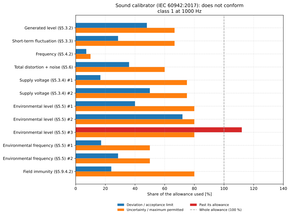
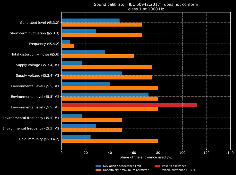
result.plot() on a pattern-evaluation record with every requirement in it.
One pair of bars per measurement: the deviation as a share of the acceptance
limit on its side, and the uncertainty as a share of the maximum permitted. A
measurement conforms when both bars stop at or before the dashed line, and a
bar whose criterion fails is drawn in red, as the legend says. Here one
environmental reading, 0.28 dB against 0.25 dB, is the whole verdict.
Show the code for this figure
import matplotlib.pyplot as pltfrom phonometry import metrology
record = metrology.SoundCalibratorMeasurements(    level_deviation_db=0.12, level_uncertainty_db=0.10,    fluctuation_db=0.02, fluctuation_uncertainty_db=0.02,    frequency_deviation_percent=-0.05, frequency_uncertainty_percent=0.02,    distortion_percent=0.9, distortion_uncertainty_percent=0.3,    supply_voltage_deviation_db=[0.01, -0.03], supply_voltage_uncertainty_db=0.03,    environmental_level_deviation_db=[0.10, -0.18, 0.28],    environmental_level_uncertainty_db=0.12,    environmental_frequency_deviation_percent=[0.12, -0.20],    environmental_frequency_uncertainty_percent=0.10,    field_immunity_deviation_db=0.06, field_immunity_uncertainty_db=0.04,)result = metrology.verify_sound_calibrator("1", record, nominal_frequency_hz=1000.0)print(result.failed)                                     # ('environmental_level',)result.plot()plt.show()
The tables. Every limit is read from a published, read-only table:
LEVEL_ACCEPTANCE_LIMITS_DB and FLUCTUATION_ACCEPTANCE_LIMITS_DB (Table 2),
SUPPLY_VOLTAGE_ACCEPTANCE_LIMITS_DB (Table 3),
FREQUENCY_ACCEPTANCE_LIMITS_PERCENT (Table 4),
ENVIRONMENTAL_LEVEL_ACCEPTANCE_LIMITS_DB (Table 5),
ENVIRONMENTAL_FREQUENCY_ACCEPTANCE_LIMITS_PERCENT (Table 6),
DISTORTION_ACCEPTANCE_LIMITS_PERCENT (Table 7) and the six maximum
uncertainties of Annex A beside them. A row of a table keyed by frequency keeps
which ends of its printed range it includes, because the page writes “31,5 to
63” in one row and ”> 63 to < 160” in the next, and a dash stays None. Classes
LS and 2 are specified from 160 Hz to 1.25 kHz only, and 5.1.2 forbids stating
conformance where the standard gives no limit, so at any other nominal
frequency the verifier refuses the class rather than borrowing a neighbour’s
row. One call judges one setting: a calibrator with several frequencies is
verified once per frequency.
Pistonphones need their correction as an input. A class LS/M or 1/M pistonphone meets its class only once the manufacturer’s static-pressure correction is applied (5.1.5), and that correction depends on the barometer reading and on data only the manual has. It goes into the record, and is added to the measured level before the level is graded (5.3.2, B.4.3.2). Every other calibrator shall need no correction at all (5.1.7), and is refused one:
from phonometry import metrology
# The level measured at the laboratory's pressure, and the manual's correction# to the reference 101.325 kPa for the barometer reading of the day.piston = metrology.SoundCalibratorMeasurements(    level_deviation_db=0.31, level_uncertainty_db=0.08,    static_pressure_correction_db=-0.12,)result = metrology.verify_sound_calibrator("1/M", piston, nominal_frequency_hz=250.0)print(f"{result.requirement('level').verifications[0].deviation:.2f}")   # 0.19print(result.passes)                                                      # True
The abbreviated environmental test. A.6.4 lets a laboratory replace the
temperature and humidity sweeps with a few combined conditions judged against
tighter limits: Table 5 less 0.05 dB for classes LS and 1 and less 0.10 dB for
class 2, and 0.5 %, 0.5 % and 1.3 % for the frequency (A.6.4.7).
environmental_test="abbreviated" applies them. A calibrator that fails them
is not thereby non-conforming: the full tests of A.6.5 to A.6.7 are then due
(A.6.1.2), which is what a failed abbreviated verdict means.
What the verdict is not. Full conformance needs the model to pass the pattern evaluation of Annex A and the specimen to pass the periodic tests of Annex B (5.1.18), and a periodic certificate says which it rests on (B.6 g and h). The requirements that are not a number with a tolerance, the markings and manual of Clause 6, the stabilization time of 5.1.10, the supply indicator of 5.7, the radio-frequency emissions of 5.9.2 and the electrostatic discharges of 5.9.3, are hardware and paperwork checks outside the verdict.
Digital analysis (dBFS)
Section titled “Digital analysis (dBFS)”If you are working with digital audio files (e.g., WAV, FLAC) and want to
analyze levels relative to Full Scale rather than physical pressure, you can use
the dbfs=True parameter.
In this mode:
- 0 dBFS corresponds to a numeric signal level of 1.0 (RMS or Peak).
- The calibration factor does not apply (dBFS is relative to digital full scale).
- Useful for analyzing headroom, digital mastering, or normalized signals.
import numpy as npfrom phonometry import filters
fs = 48000# recording: the mic capture you want to calibrate, same input chain (Pa after calibration).#   Synthesized here; in a real measurement this is your recorded signal.recording = 0.2 * np.sin(2 * np.pi * 1000 * np.arange(fs) / fs)
# Assume 'recording' is normalized between -1.0 and 1.0filtered = filters.octave_filter(    recording, fs, calibration=filters.LevelCalibration(dbfs=True))spl_dbfs, freq = filtered.levels, filtered.frequencies# Results will be negative (e.g., -20 dBFS)
The convention differs from AES17 by 3.01 dB
Section titled “The convention differs from AES17 by 3.01 dB”This is the RMS-referenced convention: a signal whose RMS is 1.0 reads
0 dBFS, so a full-scale sine, whose RMS is 0.707, reads −3.01 dBFS in
mode='rms'. AES17 (and the meters, DAWs and loudness tools that follow it)
normalise a full-scale sine to 0 dBFS instead, so the same file measured by
two tools differs by exactly 3.01 dB with neither of them wrong. Note that
mode='peak' with dbfs=True reads 0 dBFS for that same sine, because its peak
is 1.0: the RMS-versus-peak choice below and the convention question are the
same question asked twice. Any dBFS number quoted outside the library should
carry its convention with it.
What survives the loss of a physical reference
Section titled “What survives the loss of a physical reference”Half of what this library computes does not care which frame it is in, and the other half is silently meaningless without . The dividing line is whether the quantity is built from a ratio or a shape (invariant) or from an absolute value (not).
Frame-invariant (the same number in dBFS as in dB SPL): reverberation times
and decay slopes, transfer functions and coherence, correlation and delay,
spectral slopes and shapes, band-to-band differences, and any A-minus-C or
C-minus-Z difference. These are the quantities you can legitimately get from an
uncalibrated recording, and most of signals/spectra lives here.
Frame-dependent (plausible, wrong, and silent without a calibration): against a limit, SEL, noise dose and exposure, the percentile levels , every psychoacoustic quantity anchored to 20 µPa (loudness in sones, sharpness, the ECMA-418-2 chain), the peak criteria of hearing-conservation rules, and every conformance verdict in the library. None of these functions refuses uncalibrated samples (they cannot tell), so the frame is a decision the analyst has to record beside the result.
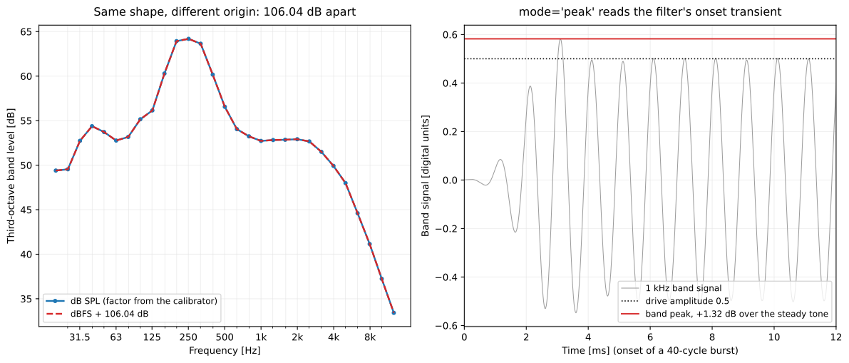
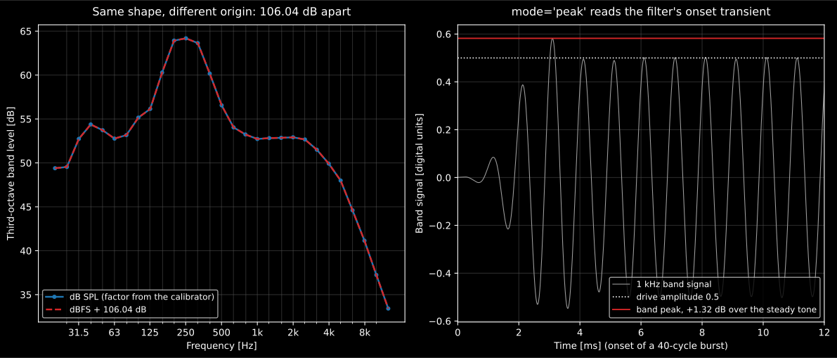
Left: one record, two frames. The dBFS spectrum is the dB SPL spectrum shifted
by a constant, here 106.04 dB, which is exactly the calibrator level minus the
dBFS level of the calibrator take: the dBFS frame changes the origin and
nothing else, which is why every shape-based quantity above survives it. Right:
the onset of a 1 kHz tone burst after the octave filter, drive amplitude 0.5.
The band signal overshoots to 0.582 before settling, so mode='peak' reads
1.32 dB above the steady tone.
RMS versus peak levels
Section titled “RMS versus peak levels”Levels can be read two ways, and both are in use in commercial analysers:
- RMS (
mode='rms') integrates energy over the frame, which is what every standardized level (, , ) is defined on. - Peak (
mode='peak') holds the largest instantaneous value in the frame, which is what impact and peak-limit criteria such as are checked against. Note that the band peak returned here is band-limited and unweighted, so it is not itself .
import numpy as npfrom phonometry import filters
fs = 48000# recording: the mic capture you want to calibrate, same input chain (Pa after calibration).#   Synthesized here; in a real measurement this is your recorded signal.recording = 0.2 * np.sin(2 * np.pi * 1000 * np.arange(fs) / fs)
# Measure peak-holding levels for impact analysisfiltered = filters.octave_filter(recording, fs, mode='peak')spl_peak, freq = filtered.levels, filtered.frequenciesInteger audio input
Section titled “Integer audio input”Integer signals (e.g. int16 from scipy.io.wavfile.read) are converted to
float64 internally before any squaring. The conversion is a dtype cast, not a
rescaling: an int16 sample of +32767 enters as 32767.0, not as 1.0. That is
harmless as long as the calibrator recording and the measurement are in the
same format, because sensitivity then returns a factor 32768 times smaller
and the two cancel exactly: a tone that reads 87.958 dB from float arrays reads
87.958 dB from the int16 arrays of the same recordings. It is not harmless
otherwise: the same tone read uncalibrated is 87.94 dB as float and 172.14 dB as
int16, a dB offset, and applying a float-derived
sensitivity to an integer-read measurement (or the reverse) carries that offset
straight into the result with no symptom. Either keep both recordings in one
format, or divide both by the full-scale value (x / 32768.0 for int16) before
anything else.
What this guide covers
Section titled “What this guide covers”Covered
IEC 60942:2017 as far as it constrains the sensitivity factor: the principal calibrator level that
target_splassumes, the Table 2 and Table A.1 class tolerances quoted in the uncertainty discussion above, and the short-term level-fluctuation check of clause 5.3.3 against the Table 2 limit of the calibrator’s class, whichsensitivity(ref, fs=fs)runs on the reference recording. And the calibrator itself:verify_sound_calibratorgrades a laboratory’s measurements of it against every requirement of IEC 60942:2017 that has an acceptance limit and a maximum-permitted uncertainty (Tables 2 to 7, Tables A.1 to A.5, 5.9.4.2 and the reduced limits of A.6.4.7), for classes LS, 1 and 2 and the pistonphone designations LS/M and 1/M, by the conformance rule of 5.1.15.Not covered
No test of IEC 60942:2017 is performed here:
verify_sound_calibratorgrades numbers measured on hardware, and the static-pressure correction of an /M pistonphone is taken from its manual, not computed, so pass an already correctedtarget_spltosensitivity()when the manual asks for one. The markings, the stabilization time, the supply indicator, the radio-frequency emissions and the electrostatic discharges of IEC 60942 are not graded. The IEC 61672-3 periodic tests are cited as laboratory practice, not run: nothing here verifies a sound level meter or assigns it a class. The dBFS half of the page sits outside any standard and makes no physical claim.
Quick answers
Section titled “Quick answers”What calibrator level should I use to calibrate my measurement chain?
Section titled “What calibrator level should I use to calibrate my measurement chain?”The usual choice is 94 dB SPL at 1 kHz (1 Pa RMS), which is what sensitivity() assumes with its default target_spl=94.0; for a 114 dB calibrator pass 114.0. IEC 60942 requires the principal level to be at least 90 dB re 20 µPa. Record a few seconds of stable tone, because the standard specifies the generated level as a 20 s average.
How much drift between the pre and post calibration checks is acceptable?
Section titled “How much drift between the pre and post calibration checks is acceptable?”Derive the sensitivity before each measurement series and check it again at the end: a common criterion invalidates the series when the two differ by more than 0.5 dB. A healthy class 1 chain drifts a few hundredths of a dB over a session, so a half-decibel pre/post difference signals damage rather than weather. Whatever the threshold, carry the difference into the uncertainty budget rather than assuming zero.
How do I check that my calibrator conforms to IEC 60942?
Section titled “How do I check that my calibrator conforms to IEC 60942?”Take the laboratory’s results (each measured deviation with the expanded uncertainty it was measured with) into a metrology.SoundCalibratorMeasurements and call metrology.verify_sound_calibrator with the class and the nominal frequency. Each requirement is judged by the conformance rule of 5.1.15: the deviation within the Table 2 to 7 limit and the uncertainty within the Annex A maximum, both inclusive. A deviation inside its limit measured with too large an uncertainty does not conform, because 5.1.16 says such a measurement cannot demonstrate anything.
Can I calibrate a class 1 chain with a class 2 calibrator?
Section titled “Can I calibrate a class 1 chain with a class 2 calibrator?”You can, but the tolerances chain: a class 1 measurement requires a class 1 (or LS) calibrator per IEC 60942 and a class 1 meter, so a class 2 calibrator silently downgrades every derived level to class 2 accuracy, because its wider level tolerance enters the sensitivity factor directly. For reference, the class 1 tolerance limit is ±0.4 dB between 160 Hz and 1.25 kHz: the 0.25 dB acceptance limit of IEC 60942:2017 Table 2 plus the 0.15 dB maximum-permitted measurement uncertainty of Table A.1, combined as Annex D describes.
References
Section titled “References”- Audio Engineering Society. (2020). AES standard method for digital audio engineering — Measurement of digital audio equipment (AES17-2020). The full-scale-sine dBFS convention, which differs from this page's RMS-referenced convention by 3.01 dB.
- Bies, D. A., Hansen, C. H., & Howard, C. Q. (2017). Engineering noise control (5th ed.). CRC Press. https://doi.org/10.1201/9781351228152Sections 3.1.5 and 3.4 (microphone field effects and sound level meter calibration: the electrical and acoustic calibration practice this page's workflow follows). ISBN 978-1-4987-2405-0.
- International Electrotechnical Commission. (2013). Electroacoustics — Sound level meters — Part 3: Periodic tests (IEC 61672-3:2013). The laboratory verification procedure behind the recommended periodic checks.
- International Electrotechnical Commission. (2017). Electroacoustics — Sound calibrators (IEC 60942:2017). The calibrator level and class assumptions behind sensitivity() (the principal level of clause 5.3.1.3, the Table 2 acceptance limits with the Table A.1 maximum-permitted uncertainties they combine with under Annex D) and the short-term level-fluctuation stability check of the reference recording (clause 5.3.3, Table 2 limits per class and nominal frequency), and every requirement with an acceptance limit and a maximum-permitted uncertainty that verify_sound_calibrator grades a calibrator against (Tables 2 to 7 and A.1 to A.5) by the conformance rule of clause 5.1.15.