Special Weightings (G, B, D, AU)

Beyond A, C and Z, the weighting family keeps four special-purpose curves, each the right tool for a narrower job: the G curve of ISO 7196:1995 rates infrasound below 20 Hz the way A-weighting rates audible noise, the historical B (ANSI S1.4-1983) reproduces measurements taken under older national codes, the withdrawn aircraft-noise D (IEC 537) serves comparisons with legacy data, and AU (IEC 61012), still in force like the G curve, keeps ultrasonic components out of an audible-exposure reading.

All four share the machinery of the IEC 61672-1 curves (0 dB at 1 kHz where applicable, multichannel and stateful block processing), and B, D and AU also take the high_accuracy oversampling, and G takes it too: the default G design oversamples toward 48 kHz, so its 0.25 Hz to 315 Hz range stays within about 0.05 dB whatever the input rate, while stateful block processing runs the plain design at the input rate, about a decibel low at 315 Hz at fs = 2000 and exactly on the 0 dB reference at 10 Hz. That matters exactly where G is used — infrasound is often recorded at 1 kHz or 2 kHz, where 315 Hz sits close to Nyquist and the bilinear warping grows quadratically; at audio rates the correction is negligible. As with A/C/Z, high_accuracy cannot be combined with stateful processing. The A, C and Z curves themselves, where they come from, the high_accuracy design and the class verification against IEC 61672-1 Table 3 are the subject of Frequency Weighting.

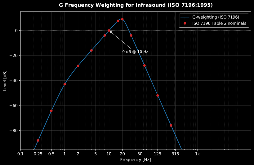
1. Infrasound: G-weighting (ISO 7196)

The G frequency weighting (ISO 7196:1995) rates infrasound the way A-weighting rates audible noise. It is defined by a pole-zero configuration normalized to 0 dB at 10 Hz, and it has three slopes, not two. Above 20 Hz the response falls at 24 dB/octave, which keeps audible-range energy out of an infrasound reading; between about 1 Hz and 20 Hz it rises at 12 dB/octave, following the steep growth of infrasound perception; and below about 1 Hz it rolls off again at 24 dB/octave, rejecting the near-static pressure fluctuations — wind loading, barometric drift, building sway — that a microphone records and nobody hears. Use it for sources with significant energy below 20 Hz (wind turbines, HVAC, blasting):

import numpy as np
from phonometry import filters

# recording: a calibrated microphone capture (Pa) — recorded through your measurement chain. Synthesized here so the guide runs standalone.
fs = 48000
recording = 0.2 * np.sin(2 * np.pi * 1000 * np.arange(fs) / fs)

g_weighted = filters.weighting_filter(recording, fs, curve='G')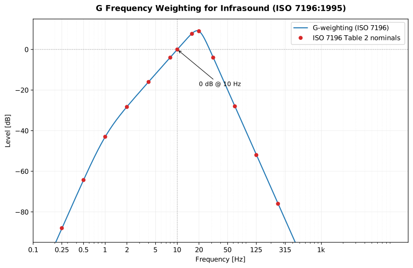

Show the code for this figure

import matplotlib.pyplot as plt
import numpy as np
from phonometry import filters

# Measure the G response: weight a centered unit impulse and take its
# spectrum. A long buffer gives the resolution the infrasound range
# needs (20 s -> 0.05 Hz).
fs = 4000
impulse = np.zeros(20 * fs)
impulse[impulse.size // 2] = 1.0
freqs = np.fft.rfftfreq(impulse.size, 1 / fs)
spectrum = np.fft.rfft(filters.weighting_filter(impulse, fs, curve="G"))

fig, ax = plt.subplots(figsize=(9, 5))
ax.semilogx(freqs[1:],
            20 * np.log10(np.abs(spectrum[1:]) + np.finfo(float).eps))
ax.plot(10, 0, "o", color="tab:red", label="0 dB at 10 Hz")
ax.set(xlim=(0.1, 1000), ylim=(-90, 15),
       xlabel="Frequency [Hz]", ylabel="G-weighting response [dB]")
ax.grid(True, which="both", alpha=0.3)
ax.legend()
plt.show()

The implementation follows the ISO 7196 Table 1 pole/zero values exactly and is verified in CI against every Table 2 nominal response value (0.25 Hz to 315 Hz). WeightingFilter(fs, "G") supports the same multichannel and stateful block processing as A/C — but stateful mode runs the plain design at the input rate, so if you stream G-weighting at a low sample rate, verify the response before trusting the level. Levels measured with the G curve are reported as $L_{pG}$ (or $L_{Geq}$ for the equivalent level over time).

Reading an LpG: the scale is not the dB(A) scale

A G-weighted level of 85 dB means nothing until you know what the scale looks like, and it does not look like the audible one. ISO 7196’s Introduction gives the anchors: the normal threshold of perception at 10 Hz is about 100 dB re 20 µPa; sounds between 1 Hz and 20 Hz that are just perceptible to an average listener yield G-weighted levels close to 100 dB; a very loud infrasound yields a G-weighted level of the order of 120 dB, only 20 dB above; and G-weighted levels below about 90 dB are not normally significant for human perception.

Two consequences follow. First, the useful range spans some 30 dB, not the 100 dB a reader is used to in dB(A), so a few decibels matter far more here — an $L_{pG}$ of 85 dB and one of 105 dB are not “similar”, they are inaudible and very loud. Second, because the growth of sensation with level is much more rapid than in the audible range while the threshold itself varies between individuals, a level near 100 dB(G) can be imperceptible to one person and clearly perceived by another, which is why infrasound complaints are investigated case by case. Compare an $L_{pG}$ against these perception anchors, never against an A-weighted limit, and never combine the two into one number.

Measuring infrasound, not just weighting it

The filter above is exact from 0.25 Hz. Almost no ordinary capture chain is, and nothing in the code can tell. ISO 7196 Annex A specifies a chain, not only a curve, and its first requirement (A.2) is a microphone with a substantially constant or well-defined frequency response over at least 0.25 Hz to 160 Hz, preferably to 315 Hz. A general-purpose measurement capsule cannot deliver that: its static-pressure equalisation vent behaves as a first-order high-pass, and a corner as high as 2 Hz already costs 7.0 dB at 1 Hz and 12.3 dB at 0.5 Hz. Any low-cut switch on the recorder removes the band being measured. The one thing that does not matter is capsule size — Annex A notes there is no practical limit on the microphone’s dimensions, because directional effects are negligible at infrasonic wavelengths.

Two actions follow. Document the chain’s own low-frequency corner and report $L_{pG}$ only down to where the chain is flat; a level quoted to 0.25 Hz from a chain that is 12 dB down at 0.5 Hz is not a measurement. Choose an averaging time long enough for the value to be representative: Annex A.5 gives an integration time or time constant of 10 s as the usual choice, 1 s when the upper part of the 1 Hz to 20 Hz band mainly contributes, and for fluctuating noise a rectangular window of at least 1 min, whose result is reported as the equivalent G-weighted sound pressure level. That is an order of magnitude longer than the 125 ms readers bring from the Fast detector.

Outdoors there is a third problem, and below 20 Hz it is usually the largest: the wind on the diaphragm generates more infrasound than the source. The microphone therefore sits at the centre of a hard board on the ground, inside a primary foam windscreen, with a secondary hemispherical screen added in wind and its insertion loss documented and corrected.

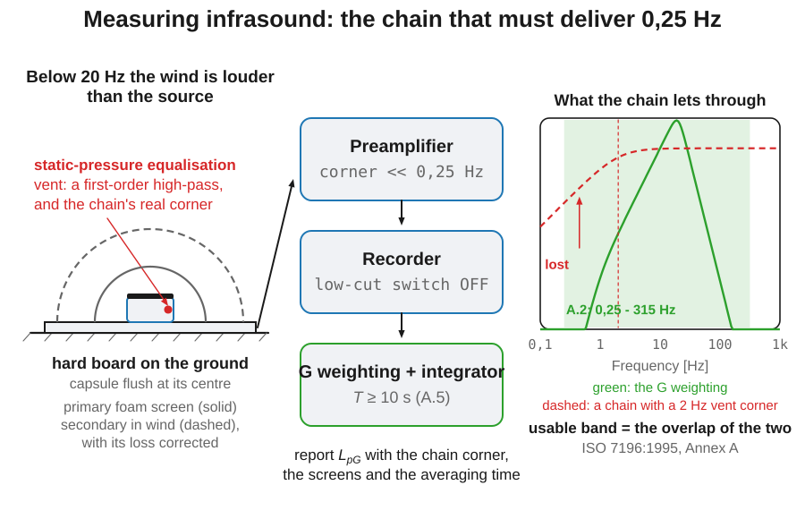
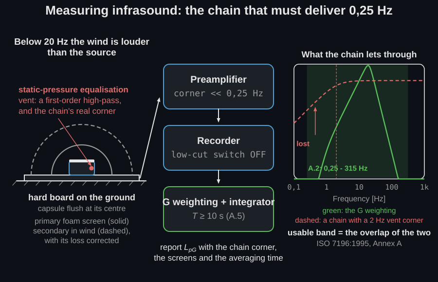
What has to be recorded for the result to be reportable is short: the chain’s own low-frequency corner, the board and the screens with their corrections, the averaging time and window shape, and the $L_{pG}$ with the analysis bandwidth it was computed over.

2. Historical and special-purpose curves: B, D and AU

Three more curves complete the family. All three work in the audible range, so they share one chart, drawn against the A curve because that is what each of them is defined or described against: B as the curve between A and C, D as the one with a hump A does not have, AU as A itself with a low-pass added.

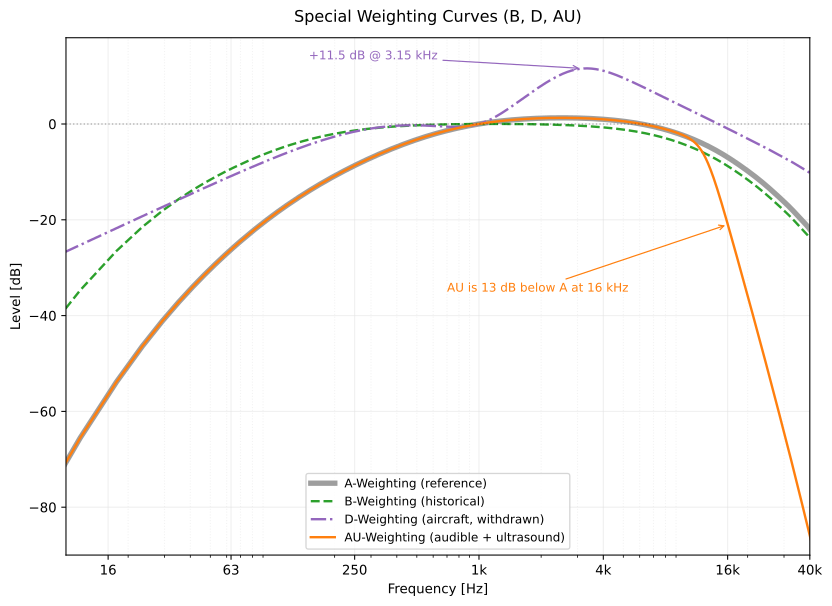
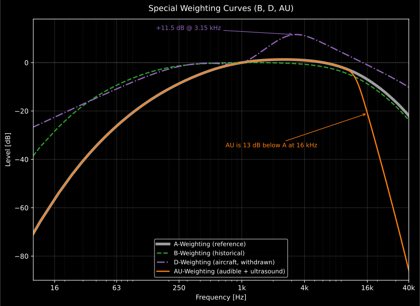
The three curves against the A reference (wide grey), measured at 96 kHz so the axis reaches the 40 kHz where IEC 61012 still specifies the U low-pass. B (green, dashed) discards less bass than A; D (purple) carries the +11.5 dB hump at 3.15 kHz where jet turbomachinery whine annoys most; AU (orange) runs inside the A reference up to 10 kHz and then falls away with U, reaching 13 dB below A at 16 kHz. The infrasound G curve keeps its own chart in section 1, and A, C and Z are in Frequency Weighting.

Show the code for this figure

import matplotlib.pyplot as plt
import numpy as np
from phonometry import filters

# Measure each curve's response: weight a centered unit impulse and take its
# spectrum. 96 kHz, not 48 kHz: it reaches the 40 kHz top row of the
# IEC 61012 U-weighting table, which is the whole point of AU.
fs = 96000
impulse = np.zeros(fs)
impulse[fs // 2] = 1.0
freqs = np.fft.rfftfreq(fs, 1 / fs)

fig, ax = plt.subplots(figsize=(9, 5))
# A goes first and wide, as the reference the other three are read against.
for curve, width in (("A", 4.0), ("B", 1.8), ("D", 1.8), ("AU", 1.8)):
    spectrum = np.fft.rfft(filters.weighting_filter(impulse, fs, curve=curve))
    ax.semilogx(freqs[1:], 20 * np.log10(np.abs(spectrum[1:]) + np.finfo(float).eps),
                label=curve, linewidth=width)
ax.set(xlim=(10, 40000), ylim=(-90, 18),
       xlabel="Frequency [Hz]", ylabel="Response [dB]")
ax.grid(True, which="both", alpha=0.3)
ax.legend()
plt.show()

B (ANSI S1.4-1983, historical)

The middle curve of the original A/B/C level-switching scheme, drawn from the ~70-phon equal-loudness contour. Analytically it is the C weighting with one more zero at the origin and one extra real pole at $f_5=158.49\text{Hz}$ (Appendix C of ANSI S1.4-1983), so it discards less bass than A and more than C. It was dropped when IEC 61672-1 replaced the older sound-level-meter standards; use it only to reproduce historical data and measurements taken under older national codes (some legacy automotive test procedures reported dB(B)). The implementation follows the ANSI S1.4-1983 Appendix C constants and is pinned in CI against the Table IV response values, within the strictest Table V mask (Type 0).

D (IEC 537, withdrawn: aircraft noise)

The D weighting approximated the perceived noisiness contours used by the perceived-noise-level (PNL) rating, so a plain sound level meter could estimate aircraft noise: the +11.5 dB hump around 3.15 kHz is where jet turbomachinery whine annoys most (it is deliberately not an equal-loudness feature). NASA’s aircraft-noise handbook gives the classic rule of thumb $L_{PN}\approx L_D+7\text{dB}$. IEC 537 was withdrawn and current certification practice reports EPNL from one-third-octave analysis or plain A-weighted levels, so D is provided for historical data and comparisons. With the standard unavailable, the implementation uses the widely published IEC 537 rational transfer function and is cross-checked against two independent implementations (SQAT’s zeros/poles and librosa’s closed form, which agree within 0.002 dB) and pinned in CI against the IEC 537 table republished in NASA CR-3406.

import numpy as np
from phonometry import filters, signals

# A 3.15 kHz whine sits right on the D-weighting hump: D rates it
# 10 dB *louder* than A does.
fs = 96000
t = np.arange(fs) / fs
whine = 0.1 * np.sin(2 * np.pi * 3150 * t)

ld = signals.leq(filters.weighting_filter(whine, fs, curve="D"))
la = signals.leq(filters.weighting_filter(whine, fs, curve="A"))
print(f"LD = {ld:.1f} dB   LA = {la:.1f} dB")
# LD = 82.5 dB   LA = 72.2 dB

AU (IEC 61012, current: audible sound in the presence of ultrasound)

The only one of the three still in force. AU is the A weighting cascaded with the U low-pass filter of IEC 61012:1990 (six poles, Table 2): flat relative to A up to 10 kHz, then a steep cutoff (-13 dB at 16 kHz, -61.8 dB at 40 kHz for U alone). Use it when strong ultrasonic components (ultrasonic cleaners and welders, rodent repellers, some public-space deterrents) would otherwise leak into an A-weighted reading through the meter’s imperfect high-frequency roll-off and overstate the audible exposure:

import numpy as np
from phonometry import filters, signals

# 1 kHz tone (audible) buried under a strong 25 kHz ultrasonic component.
fs = 96000
t = np.arange(fs) / fs
audible = 0.1 * np.sin(2 * np.pi * 1000 * t)
x = audible + 1.0 * np.sin(2 * np.pi * 25000 * t)

la = signals.leq(filters.weighting_filter(x, fs, curve="A"))
lau = signals.leq(filters.weighting_filter(x, fs, curve="AU"))
la_ref = signals.leq(filters.weighting_filter(audible, fs, curve="A"))
print(f"LA = {la:.1f} dB   LAU = {lau:.1f} dB   audible alone = {la_ref:.1f} dB")
# LA = 78.6 dB   LAU = 71.0 dB   audible alone = 71.0 dB
# The ultrasound inflates LA by 7.6 dB; AU recovers the audible level.

Ultrasound only reaches a digital filter when the sample rate captures it, so measure at 96 kHz or more (at 48 kHz there is nothing above 24 kHz to reject); the AU design internally oversamples toward 288 kHz to keep the steep U roll-off accurate. Levels are reported as $L_{AU}$. The implementation follows the Table 2 pole locations exactly (they reproduce every Table 1 nominal value within 0.05 dB) and is verified in CI against the Table 1 tolerances up to 40 kHz.

The sample rate is only the second requirement. The first is the microphone, and the arithmetic above holds only if the capsule and the interface really delivered the 25 kHz component with a known response. IEC 61012’s Introduction puts the problem plainly: a meter whose response happens to extend to the operating frequency of the ultrasonic equipment gives inflated readings of the audible part, which is what U exists to prevent — and where the ultrasonic component itself has to be quantified, the same Introduction calls for a microphone system known to have a frequency response extending at least to that operating frequency. In practice that means a 1/4 inch or 1/8 inch capsule rather than the 1/2 inch capsule used for audible work: a 1/2 inch capsule is already rolling off and strongly directional above 20 kHz, so it, and not the U filter, would decide the reading. Check the converter too — an interface that runs at 96 kHz but anti-alias filters at 20 kHz measures nothing to reject. And because the near field of a cleaner or a welder changes by several decibels over a few centimetres, take the reading at the operator’s head position and record it. Report $L_{AU}$ together with the unweighted level of the ultrasonic component and the capsule type: separating those two is the entire point of the AU weighting.

3. Class verification: B and AU yes, G and D no

Only two of the four curves on this page can return a class verdict, because only two have published tolerance tables. The verify_weighting_class verifier, described in section 6 of Frequency Weighting, also covers the curves of this guide that have published tolerance tables. For B it uses ANSI S1.4-1983 (Table IV design goals, Table V limits) and the “class” verdicts read as the standard’s instrument Types 1 and 2. For AU it uses IEC 61012:1990 Table 1 (nominal A + nominal U with the separate-unit tolerances, zero at the 1 kHz reference); IEC 61012 publishes a single tolerance set, so both margin slots agree and the verdict is simply complies (1) or not (None) — note that checking the rows above 20 kHz needs fs ≥ 96 kHz (below that they are dropped and the verdict is range_limited). G and D are rejected: ISO 7196 defines one ±1 dB tolerance with no class structure, and the withdrawn IEC 537 left no tolerance table behind (both curves are pinned numerically in the CI conformance report instead).

What this guide covers

• Covered

  ISO 7196:1995 for the G curve (Table 1 pole/zero values, verified against every Table 2 nominal response). ANSI S1.4-1983 for the historical B curve (Appendix C definition, Table IV design goals, Table V tolerance limits). IEC 61012:1990 for AU (the U low-pass of Table 2 cascaded with A, verified against Table 1). IEC 537:1976 for the withdrawn aircraft-noise D curve, implemented from its published transfer function and cross-checked against two independent implementations.

• Not covered

  verify_weighting_class does not produce a class verdict for G or D: ISO 7196 defines a single ±1 dB tolerance with no class structure, and the withdrawn IEC 537 left no tolerance table behind. Both curves are pinned numerically against their published tables in the CI conformance report instead, not through this public verifier. B and D are provided for historical data and older national codes only; neither is current practice (IEC 61672-1 replaced B, and aircraft-noise certification now reports EPNL or plain A-weighted levels instead of D).

See also

• Frequency Weighting: the A, C and Z curves, the high_accuracy design and the IEC 61672-1 Table 3 class verification these curves build on.
• API reference: filters.weighting and filters.compliance.
• Theory: G-weighting (ISO 7196): the G curve of ISO 7196 and where its normalisation comes from.

Quick answers

Which weighting should I use for infrasound below 20 Hz?

Use the G frequency weighting of ISO 7196:1995, which rates infrasound the way A-weighting rates audible noise. Normalized to 0 dB at 10 Hz, it rises at 12 dB/octave between about 1 Hz and 20 Hz, falls at 24 dB/octave above 20 Hz and rolls off again at 24 dB/octave below about 1 Hz. Apply it to sources such as wind turbines, HVAC and blasting, and report levels as $L_{pG}$ (or $L_{Geq}$ for the equivalent level over time). Read the result against the ISO 7196 perception anchors, never against an A-weighted limit: about 100 dB(G) is the normal threshold, below about 90 dB(G) infrasound is not normally significant, and a very loud infrasound is about 120 dB(G).

References

• American National Standards Institute. (1983). Specification for Sound Level Meters (ANSI S1.4-1983). The historical B weighting: Appendix C analytic definition (Formula C2), Table IV design goals and Table V tolerance limits checked by verify_weighting_class in section 3.
• Bennett, R. L., & Pearsons, K. S. (1981). Handbook of Aircraft Noise Metrics (NASA CR-3406). NASA. Republishes the IEC 537 D-weighting table (Table SLD-I) used to pin the D response in CI.
• International Electrotechnical Commission. (1976). Frequency weighting for the measurement of aircraft noise (D-weighting) (IEC 537:1976 (withdrawn)). The D weighting, implemented from its published rational transfer function and cross-checked against two independent implementations and the tabulated curve republished in NASA CR-3406 (Table SLD-I).
• International Electrotechnical Commission. (1990). Filters for the measurement of audible sound in the presence of ultrasound (IEC 61012:1990). The AU weighting: U-weighting pole locations (Table 2), nominal responses and tolerances (Table 1) and the combined AU definition of subclause 2.2.
• International Organization for Standardization. (1995). Acoustics — Frequency-weighting characteristic for infrasound measurements (ISO 7196:1995). The G-weighting pole/zero definition (Table 1), verified against every Table 2 nominal response value (0.25 Hz to 315 Hz).