Block Processing

Standards: IEC 61260 IEC 61672Key references: Oppenheim & Schafer 2010

Some measurements never fit in memory: an hour-long environmental recording, a live monitor that must report levels while the microphone is still capturing, or an embedded logger that only ever sees one buffer at a time. In all of these the signal has to be processed block by block, and the filters must behave exactly as if they had seen the whole signal at once.

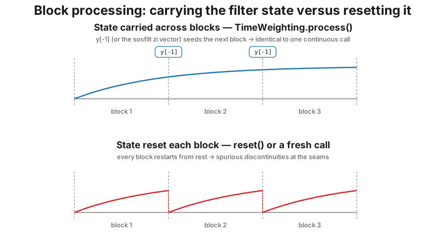
Two lanes comparing block processing with the filter state carried across blocks, giving one continuous envelope, versus reset each block, where the envelope restarts from zero at every seam

The OctaveFilterBank, WeightingFilter (any weighting curve: A, C, Z and the special B, D, G and AU) and TimeWeighting classes support block (streaming) processing: the internal filter state is carried between calls, so concatenated block outputs match a single full-signal pass. Streaming always uses the legacy bilinear weighting design — the oversampled high_accuracy path resamples internally and cannot be split across blocks — so a streamed A-weighting carries the plain-design high-frequency error described in Frequency Weighting, and a streamed G-weighting at a low sample rate loses the internal oversampling its design normally applies (see Special Weightings).

Stateful block processing matching the continuous result versus independent blocks restarting the filter transient at each boundary

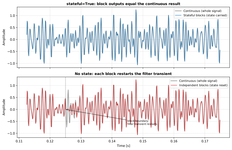
With stateful=True the concatenated block outputs match the continuous result exactly; without state, every block boundary restarts the filter transient.

A stateful bank is necessarily a different bank, and the figure’s own code says so twice: both the streamed and the offline bank are built with design=FilterDesign(resample=False). Decimation cannot carry state across blocks, so every band of a streaming bank runs at the input rate, and the offline pass it is compared against has to be built the same way. Compare a streamed result against the default octave_filter(x, fs, fraction=3) instead and you will see a residual: measured on 4 s of pink noise at 48 kHz, the two designs differ by at most 0.083 dB, with a median of 0.007 dB and the largest differences in the low bands (0.083 dB at 50 Hz). That is expected, not a bug, and it does not change the class — but if you are validating a streaming pipeline, build both sides the same way or you will be chasing the design difference instead of the state carry.

Show the code for this figure

import matplotlib.pyplot as plt
import numpy as np
from phonometry import filters

# 1 kHz octave band: four stateful blocks vs one continuous pass
fs, block = 8000, 1000
rng = np.random.default_rng(42)
x = rng.standard_normal(4 * block)
t = np.arange(x.size) / fs

bank = filters.OctaveFilterBank(
    fs, fraction=1, limits=[900, 1100],
    design=filters.FilterDesign(resample=False),
    block_processing=filters.BlockProcessing(stateful=True),
)
streamed = np.concatenate([
    bank.filter(x[i * block:(i + 1) * block], sigbands=True,
                detrend=False, calculate_level=False)[2][0]
    for i in range(4)
])
offline = filters.OctaveFilterBank(
    fs, fraction=1, limits=[900, 1100],
    design=filters.FilterDesign(resample=False),
).filter(x, sigbands=True, detrend=False, calculate_level=False)[2][0]
print(np.max(np.abs(streamed - offline)))     # 0.0 (bit-exact)

fig, ax = plt.subplots(figsize=(9, 4.5))
ax.plot(t, offline, linewidth=2.5, alpha=0.35, label="Continuous (whole signal)")
ax.plot(t, streamed, label="Stateful blocks (state carried)")
ax.axvline(block / fs, color="gray", linestyle=":", label="Block boundary")
ax.set(xlim=(0.11, 0.17), xlabel="Time [s]", ylabel="Amplitude")
ax.legend()
plt.show()

Create a stateful filter bank with block_processing=BlockProcessing(stateful=True). The internal state is zero-initialized by default but may be initialized for step-response steady-state (like scipy.signal.sosfilt_zi) with BlockProcessing(steady_ic=True). The options that must be disabled in stateful mode are summarized in the constraints table at the end of this guide.

Example: streaming a WAV file block by block

This example streams a WAV file with soundfile, an optional dependency (pip install soundfile). Any block source works just as well: scipy.io.wavfile plus manual slicing, or a live capture callback.

import soundfile as sf
from phonometry import filters

fs = 48000
octave_filter = filters.OctaveFilterBank(
    fs, 1,
    design=filters.FilterDesign(resample=False),
    block_processing=filters.BlockProcessing(stateful=True),
)
afilter = filters.WeightingFilter(fs, "A", stateful=True)

for block in sf.blocks("measurement.wav", blocksize=256, overlap=0):

    # Apply A-filter
    weighted = afilter.filter(block)

    # Split into octave bands
    block_spl, _, block_output = octave_filter.filter(weighted, sigbands=True, detrend=False)

    # further signal processing
    ...

Accumulating a level across blocks

The commonest streaming task is the one the pitfalls above say is easy: the $L_{e q}$ , or the band spectrum, of a recording that does not fit in memory. It is easy, and it is exact rather than approximate, because $L_{e q}$ has no time constant and no detector — only a sum of squares and a sample count:

total_square, n_samples = 0.0, 0

for x in audio_stream(block):        # your capture callback
    total_square += float(np.sum(np.square(x)))
    n_samples += x.shape[-1]

leq = 10 * np.log10(total_square / (n_samples * (2e-5) ** 2))

Two traps sit in those four lines. Weighting each block equally — averaging the per-block mean squares — is only correct when every block has the same length, and the last one usually does not; accumulate the sum and the count separately, as above, and the arithmetic takes care of it. And never average the per-block decibel readings: that is the arithmetic-mean error of Integrated and Statistical Levels, it is one-sided, and it always under-reads.

The band version is the same accumulator with a vector on the left:

band_squares = np.zeros(bank.num_bands)   # from your stateful OctaveFilterBank

for x in audio_stream(block):
    _, _, bands = bank.filter(x, sigbands=True, detrend=False,
                              calculate_level=False)
    band_squares += np.sum(np.square(bands), axis=-1)

Percentiles do not accumulate this way. Stream the envelope, keep it, and compute the percentiles once on the pooled result.

Time weighting across blocks

Use the TimeWeighting class (state carried automatically):

from phonometry import filters

tw = filters.TimeWeighting(fs, mode="fast")
# audio_blocks: successive frames of your microphone recording (Pa),
#   e.g. from sf.blocks("measurement.wav", ...) as in the block above.
for block in audio_blocks:
    envelope = tw.process(block)

Or manage the state yourself with the functional API; see Time Weighting.

Multichannel state

All stateful classes handle multichannel input (channels, samples): the state is allocated lazily on the first call to match the channel count, and reallocated if the channel count changes (e.g. switching from stereo to mono resets the state).

What the carried state is

Every filter in the library runs as a cascade of second-order sections in transposed direct form II. For one section with coefficients $(b_{0}, b_{1}, b_{2}, a_{1}, a_{2})$ :

y [n] = b_{0} x [n] + z_{1} [n - 1], z_{1} [n] = b_{1} x [n] - a_{1} y [n] + z_{2} [n - 1], z_{2} [n] = b_{2} x [n] - a_{2} y [n]

The pair $(z_{1}, z_{2})$ per section is the filter’s entire memory of the past. stateful=True stores these values when a block ends and restores them when the next begins, so the recursion cannot tell where one buffer stopped and the next started: the concatenated output equals the single-pass output exactly, not approximately. The TimeWeighting detector carries even less, just its last envelope value $y [n - 1]$ , which is the same value the functional API hands back as initial_state (see Time Weighting).

Streaming pitfalls

Per-block preprocessing creates seams. Anything computed from a single block that should be global, like detrending (removing the block’s own mean) or normalization, gives each block a slightly different operation: the outputs no longer concatenate into the continuous result. This is why detrend must be False in stateful mode.
Not every metric streams. Energy metrics accumulate cleanly (a running $L_{e q}$ is a running energy sum), but rank statistics do not: the $L_{90}$ of a recording is not any combination of per-block $L_{90}$ values. Stream the envelope and compute percentiles once, on the pooled result.
The first block still carries the onset transient. State starts at rest, so the filter settles during the first instants exactly as in a single pass. How long that is follows from the bandwidth: a band settles in a few times $1/ B$ , and with $B = 0.231 f_{m}$ for one-third octaves that is about a second at 12.5 Hz, a tenth of a second at 125 Hz and thirteen milliseconds at 1 kHz (the record-length rule of Filter Banks). An exponential detector adds its own $5 τ$ on top: 0.6 s on Fast, 5 s on Slow. steady_ic=True starts the sections in the steady state of a step, which removes the DC-related transient but not a band-pass ring-in, so for the low bands the honest remedy is still to discard the first seconds of the stream once (not once per block). In practice: start the logger a few seconds before the interval you intend to report.
One stream per object. A stateful instance holds the memory of one signal; feeding two interleaved streams through it corrupts both. Create one filter object per stream: the design cost is paid once at construction, not per block.
A lost or repeated buffer voids the guarantee silently. Bit-exactness assumes the blocks really were consecutive. Count blocks or compare the device timestamps, and mark the gap in the output rather than pretending the stream was continuous.
Design the filters at the rate the device actually opened, not the rate you asked for. Read the stream’s sample rate back at start-up and assert it once; a bank designed for 48 kHz fed 44.1 kHz samples reports plausible numbers for the wrong bands.
Clipping has to be detected per block. The loop replaces the instrument’s overload indicator, so test each block for runs at full scale and report a flagged block as invalid rather than averaging it in.
An unattended logger needs its own bookkeeping: a calibrator tone at the start and the end of the deployment, and a fixed level-storage interval.

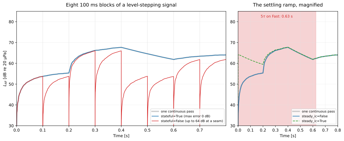
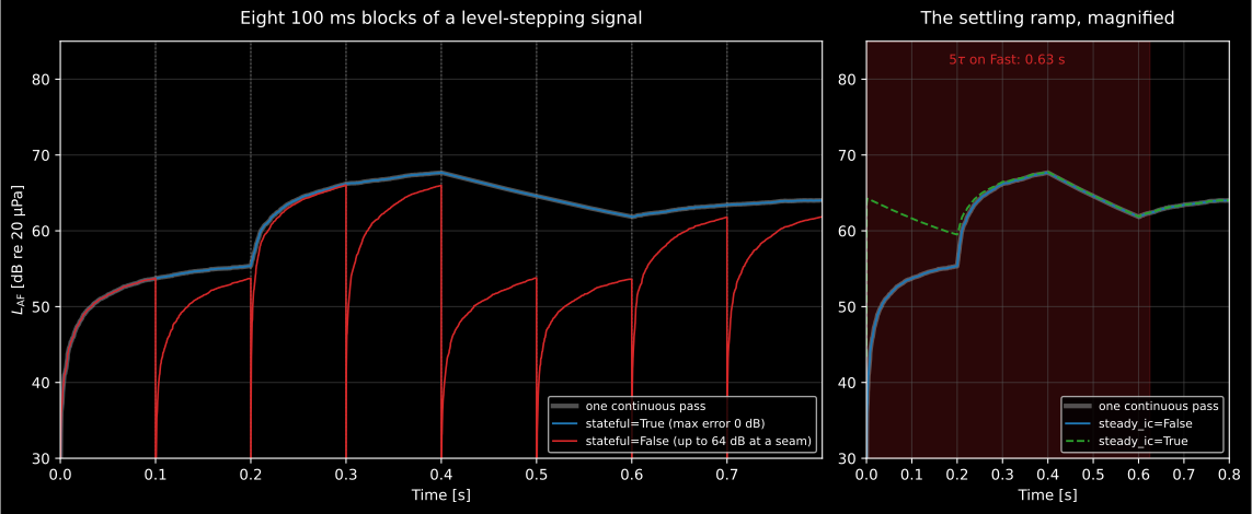
Two panels of A-weighted Fast level against time. Left, eight 100 ms blocks of a level-stepping noise: the continuous single-pass trace and the stateful streamed trace lie exactly on top of each other with a maximum error of 0 dB, while the stateless trace collapses to 30 dB at every block boundary and climbs back through the detector ramp, up to 64 dB below the true level at a seam. Right, the same first 0.8 s magnified with the first 0.63 seconds shaded: the steady_ic False trace climbs from 30 dB through the settling ramp while the steady_ic True trace starts near 64 dB, and the two converge once the ramp is over

The pitfalls above, in the domain a streaming reader actually watches. Carried state costs nothing and gains everything: the blue trace is the grey one. Reset per block and every seam becomes a fresh detector ramp — tens of decibels, at a rate set by the block length rather than by the sound. The right panel is the third pitfall: the first $5 τ$ belongs to the detector, steady_ic=True starts elsewhere rather than at the truth, and neither of them is the level until the ramp is over.

Show the code for this figure

import matplotlib.pyplot as plt

fs, block = 48000, 4800                      # 100 ms blocks
rng = np.random.default_rng(17)
x = np.concatenate([a * rng.standard_normal(block)
                    for a in (0.02, 0.02, 0.08, 0.08, 0.02, 0.02, 0.05, 0.05)])
n_blocks = x.size // block


def to_db(env):
    return 10 * np.log10(np.maximum(env, 1e-16) / (2e-5) ** 2)


# The reference has to use the design streaming can use: high_accuracy=False.
reference = to_db(filters.time_weighting(
    filters.weighting_filter(x, fs, curve="A", high_accuracy=False), fs,
    mode="fast"))

aw = filters.WeightingFilter(fs, "A", stateful=True)
tw = filters.TimeWeighting(fs, mode="fast")
streamed = np.concatenate([to_db(tw.process(aw.filter(
    x[i * block:(i + 1) * block]))) for i in range(n_blocks)])
print(f"max |streamed - continuous| = {np.max(np.abs(streamed - reference)):.3g} dB")
# max |streamed - continuous| = 0 dB

plt.plot(np.arange(x.size) / fs, reference, linewidth=3, alpha=0.4)
plt.plot(np.arange(x.size) / fs, streamed)
plt.xlabel("Time [s]")
plt.ylabel("LAF [dB re 20 uPa]")
plt.show()

Real-time level meter pattern

The canonical streaming loop weights, envelopes and reports block by block, carrying all state across calls:

import numpy as np
from phonometry import filters

fs, block = 48000, 4800  # 100 ms blocks
aw = filters.WeightingFilter(fs, "A", stateful=True)
env = filters.TimeWeighting(fs, mode="fast")  # the class is inherently stateful

laf_max = -np.inf

for x in audio_stream(block):            # your capture callback
    y = env.process(aw.filter(x))
    spl = 10 * np.log10(y[..., -1] / (2e-5) ** 2)  # instantaneous LAF
    laf_max = max(laf_max, 10 * np.log10(y.max() / (2e-5) ** 2))
    display(spl)

y[..., -1] is the detector output at the instant the block ends, so the block length is the display rate and nothing between block ends is ever observed. With a 125 ms Fast constant a block of 20 to 100 ms tracks the envelope faithfully; blocks much longer than $τ$ turn the display into a sparse sample of it. The running maximum above exists for the same reason: a peak that occurs mid-block never appears in the displayed samples, so $L_{A F ma x}$ has to be accumulated as the maximum inside each block. And the first blocks contain the detector’s own attack ramp ( $5 τ$ : 0.6 s Fast, 5 s Slow), which must be excluded from any maximum or percentile.

Stateful-mode constraints

Streaming forbids anything that needs the whole signal or that recomputes something per block. Each row below is enforced with an exception rather than silently ignored, except high_accuracy, which resolves to the legacy design unless you pass True explicitly.

Option	Stateful behavior	Why
`detrend`	must be `False`	Per-block detrending creates boundary discontinuities
`resample`	must be `False`	The resampler is not stateful
`zero_phase`	unsupported	Forward-backward filtering needs the whole signal
`high_accuracy` (weighting)	resolves to `False` by default (the legacy bilinear design, see Frequency Weighting); explicitly passing `True` raises `ValueError`	The polyphase resampling inside is block-incompatible
`steady_ic`	optional	Starts the filters in step-response steady state

What this guide covers

Covered
IEC 61260-1:2014 and IEC 61672-1:2013 exactly as far as Filter Banks, Frequency Weighting and Time Weighting already implement them: stateful=True on OctaveFilterBank, WeightingFilter and TimeWeighting carries the direct-form-II-transposed section state ( $z_{1}$ , $z_{2}$ ), or the envelope’s last value for TimeWeighting, across block boundaries, so the concatenated streamed output is bit-exact with a single full-signal pass. This page adds no normative content of its own; it only proves and documents that equivalence.
Not covered
zero_phase forward-backward filtering needs the whole signal, so it is unsupported in stateful mode; use the offline path of Filter Banks instead. high_accuracy weighting design resolves to the legacy bilinear filter in stateful mode (passing True explicitly raises ValueError), because its polyphase resampling stage is not block-compatible; see Frequency Weighting for the offline high-accuracy design. Rank statistics such as $L_{90}$ do not stream either: stream the envelope and compute percentiles once on the pooled result, as Integrated and Statistical Levels describes.

References

International Electrotechnical Commission. (2013). Electroacoustics — Sound level meters — Part 1: Specifications (IEC 61672-1:2013). The streamed frequency and time weightings are the same designs this standard governs; the carried state keeps the class and tolerance claims of the Frequency Weighting and Time Weighting pages valid in streaming use.
International Electrotechnical Commission. (2014). Electroacoustics — Octave-band and fractional-octave-band filters — Part 1: Specifications (IEC 61260-1:2014). Block processing adds no normative content of its own: the streamed octave and fractional-octave filters are the same designs this standard governs, and carrying the internal filter state across blocks is exactly what makes the concatenated output identical to a single full-signal pass, so every class and tolerance claim of the Filter Banks page holds unchanged in streaming use.
Oppenheim, A. V., & Schafer, R. W. (2010). Discrete-time signal processing (3rd ed.). Pearson. The direct-form filter structures and state recursion behind the carried state equation (ISBN 978-0-13-198842-2).

Created and maintained by José Manuel Requena Plens ORCID All projects