Time-frequency analysis

Key references: Bendat & Piersol 2010 Harris 1978

A stationary spectrum hides everything that happens in time: a passing siren, an impact, a machine running up. This page covers the two time-frequency estimators of phonometry.signals, both with the calibration discipline of the spectral-analysis page: the calibrated spectrogram (the short-time Fourier transform view of Bendat & Piersol Section 12.6.4.2, in absolute units - dB SPL for a signal in pascals) and the zoom FFT (Section 11.5.4), which computes the spectrum of a narrow band on an arbitrarily fine grid to separate tones closer than a practical full-band FFT bin. Where the levels page offers the fractional-octave-band spectrogram of a sound level meter, this one is its fine-band, constant-bandwidth counterpart.

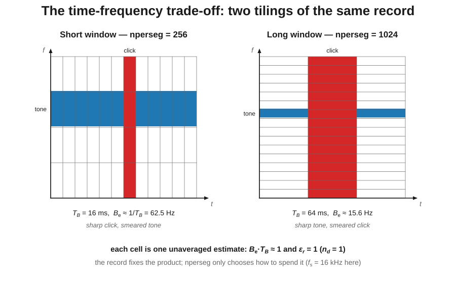
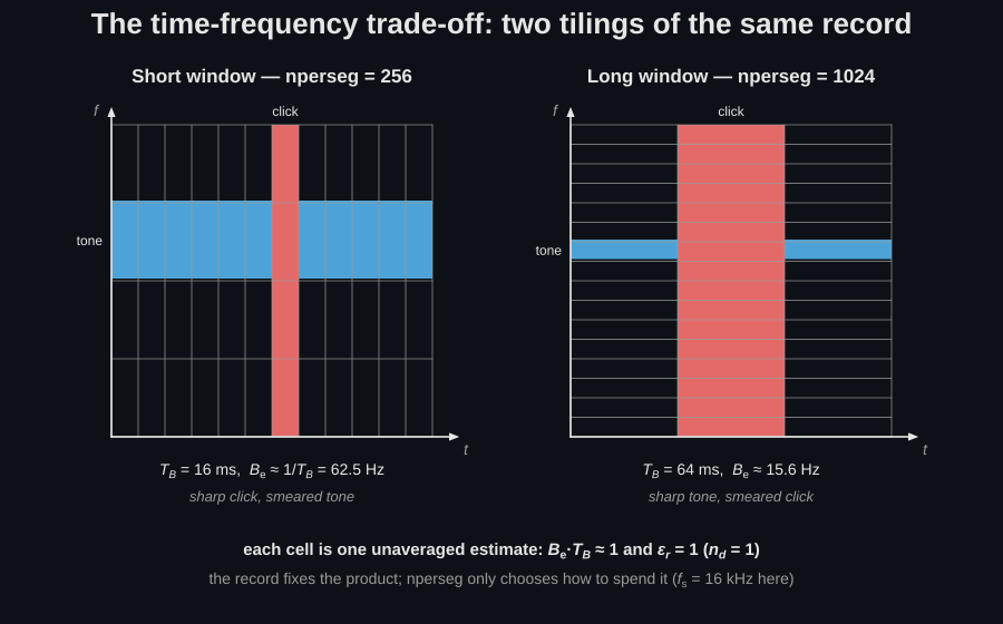
One number rules everything on this page: the segment length, which carves the time-frequency plane into cells of fixed area. The diagram shows the same record tiled by a short and a long window.

Two time-frequency plane tilings of the same record at 16 kilohertz side by side: with a short 256 sample window the cells are 16 milliseconds wide and 62.5 hertz tall, so a click stays a sharp narrow column while a steady tone smears into a tall band; with a long 1024 sample window the cells are 64 milliseconds wide and 15.6 hertz tall, so the tone sharpens into a thin band while the click smears into a wide column; captions note that each cell is a single unaveraged estimate with unit random error and that the product of time and frequency resolution stays about one

1. The calibrated spectrogram

spectrogram splits the record into tapered (Hann by default), overlapped segments - exactly the segmentation of power_spectral_density - and keeps each segment’s one-sided periodogram as one column of the time-frequency display instead of averaging them. Because the calibration is the exact Welch-module scaling with no detrending, three identities hold:

a signal in pascals yields Pa²/Hz ('density') or Pa² ('spectrum') per cell, so $10 lo g_{10} (power / p_{0}^{2})$ with 'spectrum' scaling reads a tone’s sound pressure level directly in any column it spans;
the column mean over time reproduces power_spectral_density bin by bin, with the same taper, overlap and scaling;
with a taper whose square overlap-adds to a constant (Hann at 75 % overlap), the time-integrated 'density' power equals the record’s time-domain energy exactly (Parseval plus the COLA identity - one of the conformance checks).

from phonometry import spectrogram

res = spectrogram(x, fs, nperseg=1024, overlap=0.75, scaling="spectrum")
print(res.power.shape)             # (frequencies, times)
print(res.time_resolution)         # T_B = nperseg/fs, in s
print(res.resolution_bandwidth)    # Be of the tapered segment, in Hz
res.plot()                         # dB image over the time-frequency plane

The segment length is the whole design decision: $T_{B} = nperseg / f_{s}$ of time resolution against $B_{e} = ENBW / T_{B}$ of frequency resolution, so their product $T_{B} B_{e}$ is fixed by the taper alone — 1 for a rectangular window, 1.5 for the Hann default used here (Section 12.6.4.2, and the window figures of merit on the spectral-analysis page). The tiling diagram above draws the untapered case, where that product is exactly one. Halving the segment length buys twice the time resolution and costs exactly half the frequency resolution; nothing buys both. Long segments pin frequencies and smear transients; short segments do the opposite. And because each cell is a single unaveraged estimate, random data carries a per-cell normalized random error of 1 (Eq. 8.158 with $n_{d} = 1$ ; Bendat & Piersol quote $2 /1.25 \approx 1.13$ for the magnitude display) - the spectrogram is a tool for deterministic structure (tones, sweeps, transients), while the averaged Welch estimate is the low-variance tool for the stationary background.

Put a number on that. A single periodogram cell of random data is chi-square with two degrees of freedom, so its level has a standard deviation of about 5.6 dB and a 90 % spread of roughly 17 dB — the mottled texture of the noise floor in the figure below, and the reason a single bright cell means nothing at all. The reading rule follows: a feature is real when it persists across neighbouring columns or bins, because the cell-to-cell fluctuation is independent while structure is not, so the eye is doing the averaging the estimator refused to do. Both remedies cost something: averaging adjacent columns trades time resolution for variance and converges toward the Welch estimate, and smoothing across frequency with the fractional-octave kernel of the spectral analysis page trades frequency resolution for the same thing. Which is exactly why a noise floor should be quantified from a PSD and only displayed on a spectrogram.

Choosing the segment for the event

The trade-off is fixed, so the choice has to come from the thing being measured.

For a transient, keep $T_{B}$ below the decay you want to see. The 12 ms decay of the impact in the figure below asks for segments of a few milliseconds — about 256 samples at 48 kHz — and the frequency resolution then follows at about 190 Hz, whether you wanted it or not.

For a component whose frequency moves at a rate $r$ in Hz/s, the tone leaves its own resolution bandwidth inside a single segment unless $B_{e} \geq r T_{B}$ . With $B_{e} = 1.5/ T_{B}$ that gives an optimum $T_{B} = 1.5/ r$ . The siren below sweeps at up to about 950 Hz/s, so segments shorter than 40 ms keep the ridge sharp — and the 1024-point choice at 16 kHz is 64 ms, already past it, which is why the ridge thickens at the steepest part of the sweep. A run-up sweeping a 500 Hz order at 100 Hz/s wants segments of about 0.12 s and nothing longer.

The two requirements routinely conflict, as they do in the figure’s own scene. The honest recipe: choose $T_{B}$ from the fastest thing that must stay sharp, check the resulting $B_{e}$ against the closest two components that must stay separate, and when the two cannot both be met, say so in the caption instead of splitting the difference. res.time_resolution and res.resolution_bandwidth report the pair actually delivered, so the choice can be stated in a report.

One acquisition note, because it is the failure that looks like a result: capture transients with a pre-trigger of at least one segment, fix the gain in advance and verify that no sample clips — a clipped impact draws a full-height stripe that looks exactly like a broadband event.

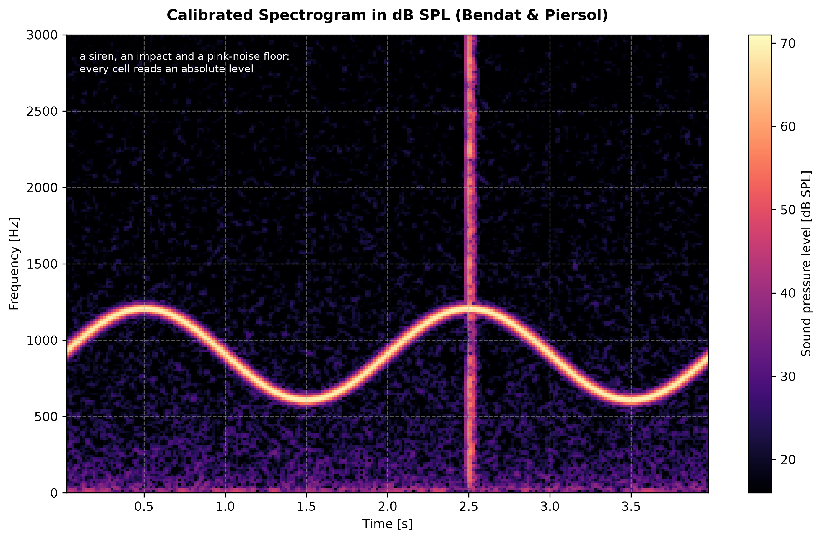
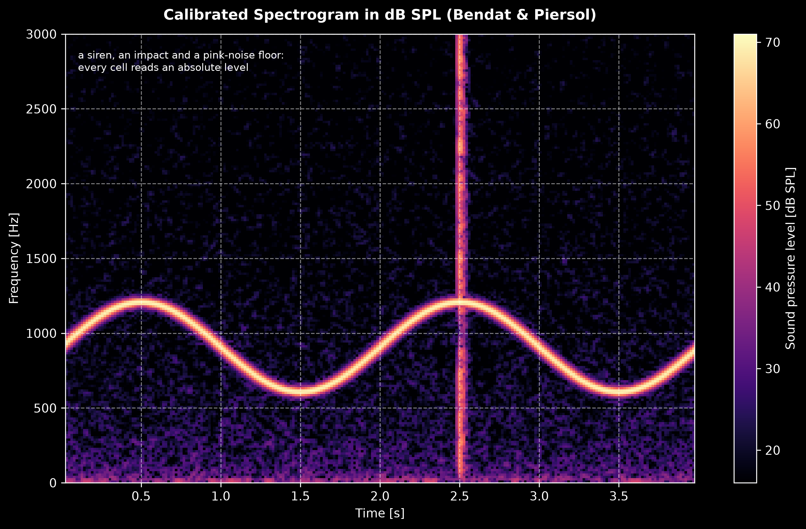
Calibrated spectrogram in dB SPL of a synthetic four-second outdoor scene: a siren sweeping sinusoidally between 600 and 1200 hertz traces a bright oscillating ridge at 70 decibels, a broadband impact at two and a half seconds draws a vertical stripe, and a pink noise background whose broadband level is 45 decibels fills the image at a much lower per-cell level, with the color bar reading absolute sound pressure level

Reading it: the siren ridge really does read 70 dB SPL, because a tone puts all its power inside one resolution bandwidth and the 'spectrum' cell is therefore its mean square. The pink background does not read 45 dB anywhere. That 45 dB is its broadband level spread over the whole band, and each cell carries only the part inside one $B_{e}$ — some 25 dB lower here, for a 1024-point segment at 16 kHz. To recover a level from noise, convert cells to a density by subtracting $10 lo g_{10} B_{e}$ and integrate over the band of interest, or use 'density' and integrate directly. And the impact’s peak cell is not the impact’s level either: a transient shorter than the segment spreads its energy over the whole column, so that reading depends on nperseg. The colour bar is an absolute scale for tonal structure and a bandwidth-dependent one for everything else; when absolute band levels over time are the goal, the band spectrogram of Levels is the right tool.

Show the code for this figure

import matplotlib.pyplot as plt
import numpy as np
from phonometry import noise_signal, spectrogram

fs = 16000.0
t = np.arange(int(4.0 * fs)) / fs
p_ref = 2e-5

siren_rms = p_ref * 10.0 ** (70.0 / 20.0)          # 70 dB SPL siren
x = siren_rms * np.sqrt(2.0) * np.cos(
    2.0 * np.pi * 900.0 * t - 600.0 * np.cos(np.pi * t)
)
rng = np.random.default_rng(9)
n_imp = int(0.06 * fs)                              # impact at t = 2.5 s
x[int(2.5 * fs):int(2.5 * fs) + n_imp] += 0.4 * (
    rng.standard_normal(n_imp) * np.exp(-np.arange(n_imp) / (0.012 * fs))
)
x += noise_signal(fs, 4.0, color="pink",            # 45 dB SPL floor
                  rms=p_ref * 10.0 ** (45.0 / 20.0), seed=10)

res = spectrogram(x, fs, nperseg=1024, overlap=0.75, scaling="spectrum")
level = 10.0 * np.log10(res.power / p_ref**2)

fig, ax = plt.subplots(figsize=(10, 6))
img = ax.imshow(level, cmap="magma", vmin=level.max() - 55.0,
                vmax=level.max(), aspect="auto", origin="lower",
                extent=(res.times[0], res.times[-1], 0.0,
                        res.frequencies[-1]))
fig.colorbar(img, ax=ax, label="Sound pressure level [dB SPL]")
ax.set_ylim(0.0, 3000.0)
ax.set_xlabel("Time [s]")
ax.set_ylabel("Frequency [Hz]")
plt.show()

res.plot() draws the same display from the result directly (a single raster image, 80 dB below the strongest cell by default; pass vmin/vmax to change the range, or ax to draw into an existing panel).

2. Zoom FFT

Two tones 3 Hz apart - gear sidebands, twin machines, mains hum against a rotor harmonic - are invisible to a 1024-point FFT at 8192 Hz: its bins are 8 Hz wide. The classical analyzer solution is the zoom transform of Bendat & Piersol Section 11.5.4: bandpass the record, shift the band down to zero frequency by complex demodulation with $exp (- j 2 π f_{1} t)$ (Eqs. 11.123-11.126), decimate by the bandwidth ratio and Fourier transform the decimated record (Eqs. 11.128-11.130), obtaining a fine bin spacing over the band without a giant FFT block (Eq. 11.127).

zoom_fft computes the exact single-pass digital equivalent - the chirp-Z evaluation of the tapered record’s DFT on the zoom grid - which yields the same DFT samples as the demodulate-decimate chain; the test suite pins the two against each other at machine precision. Amplitudes are calibrated per the taper’s coherent gain, so a sine of peak amplitude $A$ on an analysis frequency reads amplitude $= A$ and power $= A^{2} /2$ exactly:

from phonometry import zoom_fft

res = zoom_fft(x, fs, 980.0, 1016.0)     # grid at the record resolution
print(res.bin_spacing)                   # fs/N by default
print(res.resolution_bandwidth)          # Be of the tapered record
peak = res.amplitude.argmax()
print(res.frequencies[peak], res.amplitude[peak])
res.plot()                               # power spectrum in dB over the band

One distinction matters and the result states it: the grid can be made arbitrarily fine (n_points), but the resolution - the ability to separate two tones - is set by the record length and taper, reported as resolution_bandwidth ( $B_{e} = f_{s} \sum w^{2} / (\sum w)^{2}$ , i.e. $1/ T_{r}$ untapered and $1.5/ T_{r}$ for Hann — the same taper factor as section 1, applied here to the record duration $T_{r}$ rather than to a segment, because the zoom FFT transforms the whole record). Zooming refines the sampling of the same underlying spectrum; only a longer record separates closer tones.

Dynamic range is a separate question, and the zoom does not help with it. The chirp-Z still evaluates the DFT of the tapered whole record, so a strong component outside the zoom band leaks into it through the taper’s sidelobes exactly as it would in an ordinary FFT: the zoom band buys resolution of the grid, not rejection. Hann’s first sidelobe is −31.5 dB, which is nowhere near enough to see a sideband 50 dB below a carrier a few hertz away. The control is the window argument (default "hann"): pass window="blackman", or a Kaiser with a high beta, to trade main-lobe width for sidelobe rejection — remembering that the wider main lobe raises $B_{e}$ and therefore the closest spacing you can separate, so the two goals pull against each other. The window figures of merit put numbers on that trade. When even the best taper is not enough, pre-filter or notch the dominant component before zooming: no window substitutes for removing the energy.

And the machine has to hold still. Separating two lines 3 Hz apart near 1 kHz needs about a second of record, and over that second the shaft must hold its speed to better than 3 parts in 1000 — 0.3 % — or the rotor line alone smears wider than the separation you are trying to resolve, and no zoom recovers it. In general the speed stability required is the target resolution divided by the frequency of the line, which gets harsh fast: 0.5 Hz at 5 kHz is 0.01 %. Check it before you trust the zoom: run a spectrogram of the same record and confirm the line is horizontal across the analysis window, or read the shaft period from a tacho over the record. When the machine does drift, angularly resample against the tacho — order tracking — so the lines become stationary in order rather than in frequency.

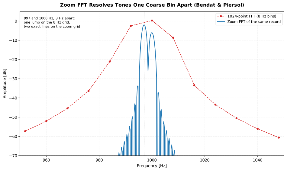
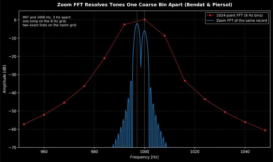
Zoom FFT of a one-second record containing tones at 997 and 1000 hertz: the coarse 1024-point FFT with 8 hertz bins shows a single broad lump, while the zoom FFT over 980 to 1016 hertz draws two separate mainlobes whose peaks sit exactly on the dotted true-tone frequencies

What separates the two tones is the second of record, not the zoom. The coarse view uses 1024 of the 8192 samples, so its 8 Hz bins cannot hold two lines 3 Hz apart and it shows one lump at 1000 Hz. The zoom transforms the whole record, whose Hann resolution bandwidth is 1.5 Hz, and puts a 0.25 Hz grid on it: the peaks land on 997.00 and 1000.00 Hz at −1.94 and −6.02 dB, the amplitudes of the two tones. A finer grid on a 1024-sample record would have changed nothing — this is the distinction the section makes between sampling density and resolution.

Show the code for this figure

import matplotlib.pyplot as plt
import numpy as np
from scipy import signal
from phonometry import zoom_fft

fs = 8192.0
t = np.arange(8192) / fs                 # 1 s record: 1 Hz resolution
x = (0.8 * np.cos(2.0 * np.pi * 997.0 * t)
     + 0.5 * np.cos(2.0 * np.pi * 1000.0 * t))

w = signal.get_window("hann", 1024)      # the coarse view: 8 Hz bins
coarse = 2.0 * np.abs(np.fft.rfft(x[:1024] * w)) / np.sum(w)
coarse_f = np.fft.rfftfreq(1024, 1.0 / fs)
band = (coarse_f >= 950.0) & (coarse_f <= 1050.0)

res = zoom_fft(x, fs, 980.0, 1016.0, n_points=145)   # 0.25 Hz grid

fig, ax = plt.subplots(figsize=(10, 6))
ax.plot(coarse_f[band], 20.0 * np.log10(coarse[band]), "o--",
        label="1024-point FFT (8 Hz bins)")
ax.plot(res.frequencies, 20.0 * np.log10(res.amplitude),
        label="Zoom FFT of the same record")
for f0 in (997.0, 1000.0):
    ax.axvline(f0, color="k", ls=":", lw=1.0, alpha=0.6)
ax.set_ylim(-70.0, 5.0)
ax.set_xlabel("Frequency [Hz]")
ax.set_ylabel("Amplitude [dB]")
ax.legend()
plt.show()

Relation to the rest of the library

The spectrogram shares its taper, segmentation and scaling with power_spectral_density, so the two are mutually consistent bin by bin; the octave-band spectrogram of OctaveFilterBank.spectrogram is the constant-percentage-bandwidth counterpart with sound-level-meter ballistics; and for tracking a single component’s frequency in time, the Hilbert instantaneous frequency of envelope complements the STFT ridge.

What this guide covers

Covered
Bendat & Piersol’s calibrated spectrogram (Section 12.6.4.2): tapered, overlapped STFT segments kept as separate time columns instead of averaged, implemented by spectrogram with the exact Welch-module scaling and the Eq. 8.158 random error of an unaveraged cell. The zoom FFT of Section 11.5.4 (Eqs. 11.122-11.130): band-limited, arbitrarily fine-grid spectra computed as the chirp-Z equivalent of the book’s demodulate-decimate-DFT chain, implemented by zoom_fft. Both share the Harris (1978) window catalogue behind the segment taper.
Not covered
This is the constant-bandwidth, STFT-based family only. The constant-percentage-bandwidth, sound-level-meter counterpart is OctaveFilterBank.spectrogram on the Levels page. Tracking a single component’s instantaneous frequency over time is the Hilbert envelope of envelope, on the Correlation and delay page, not this one. As with the spectral-analysis page, this implements Bendat & Piersol’s estimators, not a certification standard.

References

Bendat, J. S., & Piersol, A. G. (2010). Random data: Analysis and measurement procedures (4th ed.). Wiley. https://doi.org/10.1002/9781118032428Section 12.6.4.2 (spectrograms and their random errors), Section 11.5.4 (zoom transform procedures, Eqs. 11.122-11.130) and Sections 8.5.1/8.5.4 (resolution bandwidth and the statistical errors of unaveraged estimates). ISBN 978-0-470-24877-5.
Harris, F. J. (1978). On the use of windows for harmonic analysis with the discrete Fourier transform. Proceedings of the IEEE, 66(1), 51-83. https://doi.org/10.1109/PROC.1978.10837The taper catalogue behind the segment window: main-lobe width versus sidelobe leakage, the trade-off that sets what a spectrogram column can resolve at a given segment length.

Created and maintained by José Manuel Requena Plens ORCID All projects