Calibrated spectral analysis

A spectrum without its uncertainty is half a measurement. This page covers the Welch spectral estimators of phonometry.signals that report, next to the spectrum itself, the statistical quality of the estimate following Bendat & Piersol, Random Data: Analysis and Measurement Procedures (4th ed., 2010): the power spectral density and cross-spectral density with the effective number of averages, the normalized random error and chi-square confidence intervals; the coherent output spectrum that splits a measured output into the part linearly explained by the input and the noise remainder, with the spectral signal-to-noise ratio; a fractional-octave smoother with a constant-power kernel; and colored-noise generators with an exact power-law slope for exercising all of the above. A Thomson multitaper estimator (Percival & Walden, 1993) completes the family for records too short to segment. Every error formula is a closed form from the sources, verified by seeded Monte Carlo in the test suite.

1. Power spectral density with its statistical error

power_spectral_density estimates the one-sided autospectral density $G_{xx}(f)$ by Welch’s method: the record is split into tapered (Hann by default), 50 %-overlapped segments whose periodograms are averaged. No detrending is applied, so absolute calibration is preserved: a signal in pascals yields Pa²/Hz. Two scalings are available: 'density' (units²/Hz, integrates to the signal power) and 'spectrum' (units², reads the power of discrete tones directly).

The price of preserving the calibration is that any DC offset or slow drift stays in the record and leaks. The offset lands in the DC bin, and the Hann taper’s sidelobes spread a fraction of it over the first few bins, so an uncorrected offset appears as a spurious low-frequency rise that no amount of averaging removes. When the lowest bins matter, subtract the mean or high-pass the record explicitly before the call — that is a change to the signal, not a setting on the estimator — and note that the same offset is invisible in a fractional-octave display, because no band reaches DC. The same condition returns in Data qualification, whose level-crossing and peak statistics are written for a zero-mean process.

The estimator is a fixed pipeline: the window sets the resolution bandwidth, and the effective averages follow from the record length (the raw segment count) together with the window and overlap. Once those are fixed every quality figure follows from the main design choice, the segment length. The diagram traces it with the numbers of this page’s example.

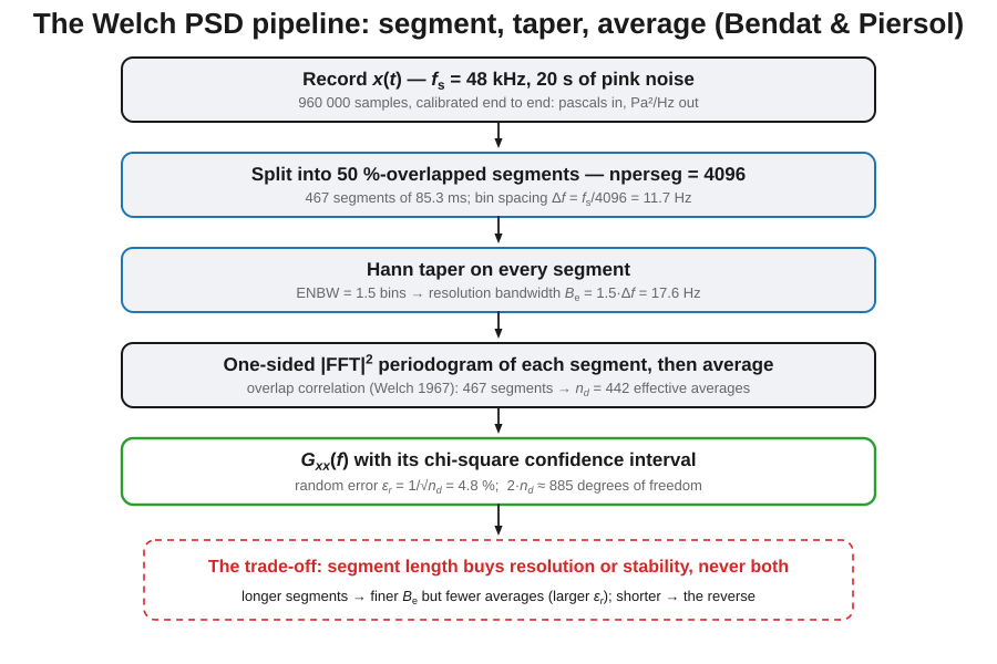
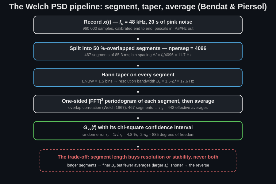
Averaging $n_d$ independent segments gives the estimate $2n_d$ chi-square degrees of freedom (Eq. 8.162), from which everything else follows:

$${\epsilon }_r[{\hat{G}}_{xx}]=\frac{1}{\sqrt{n_d}},\frac{n{\hat{G}}_{xx}}{{\chi }_{n;\alpha /2}^2}\le G_{xx}\le \frac{n{\hat{G}}_{xx}}{{\chi }_{n;1-\alpha /2}^2},n=2n_d.$$

With overlapped, tapered segments the averages are correlated, so the result reports both the raw segment count (n_segments) and the effective number of independent averages (n_averages), computed with the window-correlation formula of Welch (1967) that Bendat & Piersol reference in Section 11.5.2.2; for a Hann taper at 50 % overlap it is roughly 0.95 of the raw count. The random error and the confidence interval use the effective value. At DC, and at Nyquist for an even segment length, the one-sided spectrum has a single real Fourier component, so those bins carry half the degrees of freedom and a correspondingly wider interval.

from phonometry import power_spectral_density

# record: one channel of a calibrated capture, in pascals (see the Calibration
#   guide below); in dBFS work it is the raw [-1, 1] array and the result is
#   FS^2/Hz. fs: its sample rate in Hz.
res = power_spectral_density(record, fs)          # Hann, 50 % overlap, 95 % CI
print(res.n_averages, res.random_error)           # nd and 1/sqrt(nd)
print(res.ci_lower[10], res.psd[10], res.ci_upper[10])
res.plot()                                        # PSD in dB with the CI band

The resolution bias is the other half of the error budget: a finite analysis bandwidth $B_e$ (reported as resolution_bandwidth, the effective noise bandwidth of the taper) smooths sharp spectral features, always in the direction of reduced dynamic range (Eq. 8.139). For a resonance peak of half-power bandwidth $B_r$, the first-order normalized bias is the closed form of Eq. 8.141, exposed as resolution_bias_error:

$${\epsilon }_b[{\hat{G}}_{xx}(f_r)]\approx -\frac{1}{3}{\left(\frac{B_e}{B_r}\right)}^2.$$

from phonometry import resolution_bias_error

eps_b = resolution_bias_error(res.resolution_bandwidth, 25.0)  # Br = 25 Hz peak

Narrow $B_e$ (long segments) suppresses the bias but leaves fewer averages and a larger random error; the two requirements on segment length pull in opposite directions, which is exactly the trade-off the reported numbers make visible.

Choosing the segment length, and then the record length

The bias formula is more useful read backwards. Keeping a resonance peak’s bias under 1 dB means ${\epsilon }_b\ge -0.2$, hence $B_e\le 0.775B_r$; keeping it under a tenth of a decibel means $B_e\le 0.263B_r$. The familiar rule of thumb — three or four analysis bandwidths across the half-power width of the narrowest feature that matters — is exactly this formula, and now it has a number attached to it.

Work forward from the measurement rather than from a habitual nperseg. A mode at 100 Hz with $Q=50$ has $B_r=f/Q=2$ Hz. Holding its bias under 2 % (0.09 dB) needs $B_e\le B_r\sqrt{3\times 0.02}=0.49$ Hz, and for the Hann taper $B_e=1.5f_s/\text{nperseg}$, so at 48 kHz that is nperseg $\ge 147000$, i.e. segments of at least 3.1 s. Asking for a 10 % random error then needs $n_d=100$ effective averages, which at 50 % overlap means a record of about 150 s:

target_bias = 0.02                     # 2 % on the peak, about 0.09 dB
b_r, q = 100.0 / 50.0, 100             # a 100 Hz mode with Q = 50
b_e = b_r * (3 * target_bias) ** 0.5   # the analysis bandwidth it allows
nperseg = 1.5 * 48000 / b_e            # Hann: Be = 1.5 fs / nperseg
record_s = q * 0.5 * nperseg / 48000   # nd = 100 averages at 50 % overlap
print(round(b_e, 2), int(nperseg), round(record_s))     # 0.49 146969 153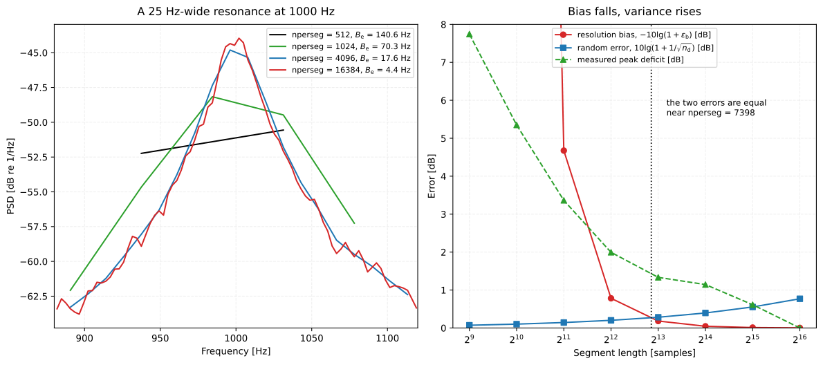

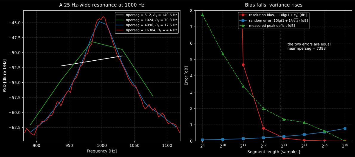
The same 25 Hz-wide resonance seen at four segment lengths. At nperseg = 512 the analysis bandwidth is 140.6 Hz, five times the resonance width, and the peak reads about 8 dB low and far too broad; by 4096 the bandwidth is 17.6 Hz and the peak is essentially resolved. The right panel puts the two errors on one axis: the bias falls as $B_e^2$ and the random error rises as $n_d^{-1/2}$, and they are equal near nperseg = 7400 for this resonance — which is the segment length to choose if there is no reason to favour one error over the other.

The two decisions are independent: the segment length is set by the sharpest feature that matters, the record length by the precision you want. Lengthening the segments without lengthening the record trades one error for the other and buys nothing. And 150 s of record is 150 s over which the process has to stay stationary — which is a claim, not an assumption, and the one Data qualification decides. When the record simply cannot be that long, the multitaper estimator of section 7 is the escape.

From digital units to dB SPL

power_spectral_density scales whatever it is given and applies no calibration of its own, so the sensitivity factor goes on the record, before the estimate:

calibration_factor = 1.002             # Pa per digital unit, from the calibrator
pressure = calibration_factor * record
psd = power_spectral_density(pressure, fs)      # now in Pa^2/Hz

The ordinate is then $10{\log }_{10}(G_{xx}/p_0^2)$ dB re (20 µPa)²/Hz, and with scaling="spectrum" the same call reads a discrete tone’s level directly as $10{\log }_{10}(P/p_0^2)$ dB. To get from there to the band level an acoustic report contains, integrate the density over the band — sum the bins and multiply by the bin spacing — and divide by $p_0^2$; fractional_octave_smoothing in section 4 is a display smoother and not a substitute for that integration, as that section spells out. The factor itself comes from Calibration and dBFS.

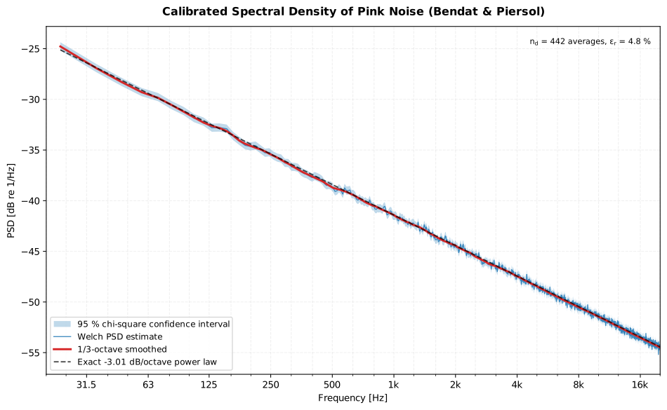
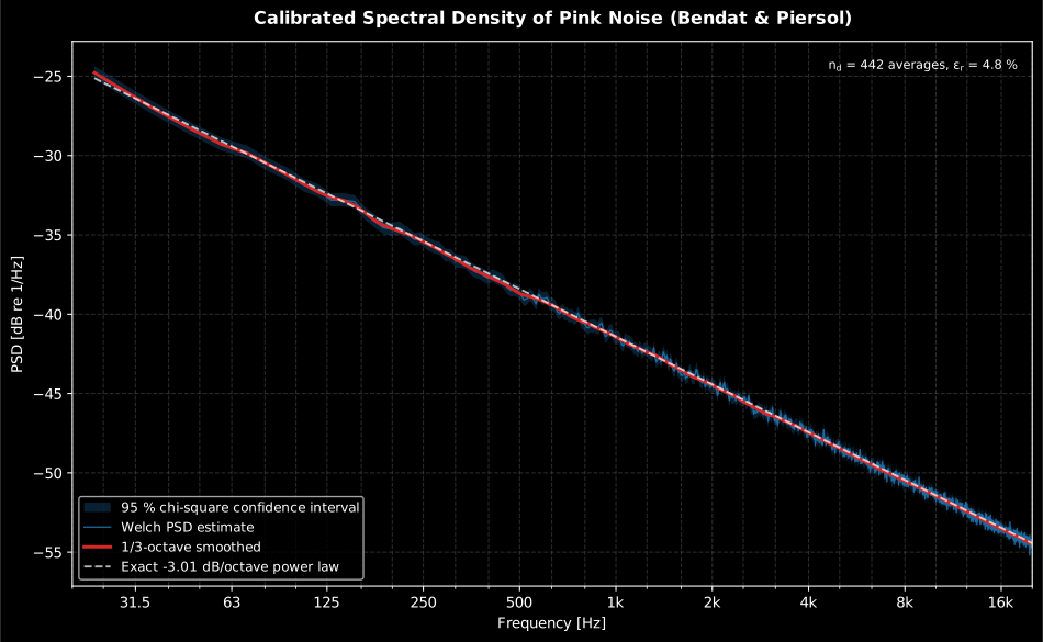
What 20 s of record buys, read off the figure. 467 segments of 4096 samples give 442 equivalent averages, a normalized random error of 0.047 and a 95 % chi-square band 0.81 dB wide — so the ragged estimate is never more than about 0.8 dB from the smoothed curve anywhere in the decade, and the shaded band, not the ripple, is the honest statement of what is known. Both curves fit −3.007 dB/octave against the exact −3.01 dB/octave of pink noise. Smoothing narrows nothing: it redraws the same estimate, and the interval below it still applies.

Show the code for this figure

import matplotlib.pyplot as plt
import numpy as np
from phonometry import (
    fractional_octave_smoothing,
    noise_signal,
    power_spectral_density,
)

fs = 48000.0
x = noise_signal(fs, 20.0, color="pink", seed=11)
res = power_spectral_density(x, fs, nperseg=4096)
band = (res.frequencies >= 20.0) & (res.frequencies <= 20000.0)
freqs = res.frequencies[band]
smooth = fractional_octave_smoothing(res.frequencies, res.psd, 3.0)[band]

fig, ax = plt.subplots(figsize=(10, 6))
ax.fill_between(freqs, 10 * np.log10(res.ci_lower[band]),
                10 * np.log10(res.ci_upper[band]), alpha=0.3,
                label="95 % chi-square confidence interval")
ax.semilogx(freqs, 10 * np.log10(res.psd[band]), lw=1.0,
            label="Welch PSD estimate")
ax.semilogx(freqs, 10 * np.log10(smooth), lw=2.2,
            label="1/3-octave smoothed")
ax.set_xlabel("Frequency [Hz]")
ax.set_ylabel("PSD [dB re 1/Hz]")
ax.legend()
plt.show()

2. Cross-spectral density

cross_spectral_density estimates the complex $G_{xy}(f)$ between two channels with the same Welch core, and reports the ordinary coherence ${\gamma }_{xy}^2=|G_{xy}{|}^2/(G_{xx}{G}_{yy})$ together with the Bendat & Piersol random errors of the magnitude and phase (Eqs. 9.33 and 9.52, with the measured coherence in place of the unknown true value, as the book recommends for measured data):

$${\epsilon }_r[|{\hat{G}}_{xy}|]=\frac{1}{|{\gamma }_{xy}|\sqrt{n_d}},s.d.[{\hat{\theta }}_{xy}]=\frac{{\left(1-{\gamma }_{xy}^2\right)}^{1/2}}{|{\gamma }_{xy}|\sqrt{2n_d}}.$$

Both shrink as the coherence approaches one: a strongly coherent pair needs far fewer averages for the same confidence. The phase is unwrapped, so its slope against frequency is the group delay ${\tau }_g=-\mathrm{d}\phi /(2\pi \mathrm{d}f)$; for a pure delay path the phase is linear and that slope reads the propagation delay directly.

from phonometry import cross_spectral_density

res = cross_spectral_density(x, y, fs)
print(res.magnitude_random_error[100], res.phase_std[100])  # bin 100 errors
res.plot()   # magnitude, phase with ±sigma band, coherence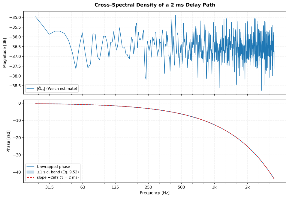

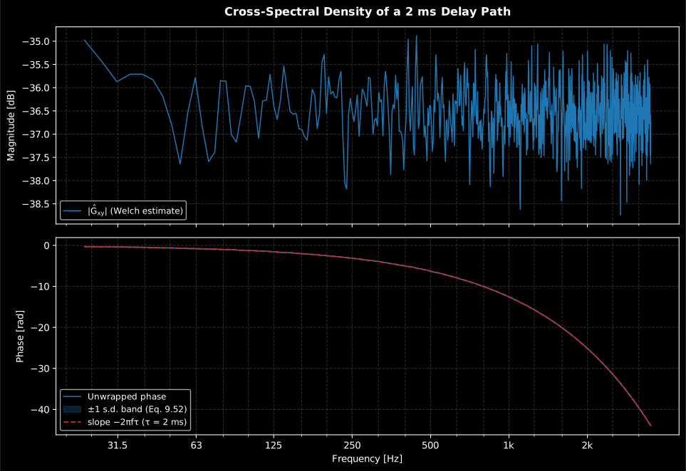
The cross-spectral density of a 2 ms delay path: the unwrapped phase is exactly the line $-2\pi f\tau$, so its slope reads the propagation delay directly, and the ±1 s.d. band of Eq. 9.52 quantifies how far to trust it per frequency.

Show the code for this figure

import matplotlib.pyplot as plt
import numpy as np
from phonometry import cross_spectral_density, noise_signal

fs = 8000.0
tau = 0.002                                   # 2 ms = 16 samples
delay = int(tau * fs)
x = noise_signal(fs, 8.0, seed=8)
noise = noise_signal(fs, 8.0, rms=0.3, seed=9)
y = 0.9 * np.concatenate([np.zeros(delay), x[:-delay]]) + noise

res = cross_spectral_density(x, y, fs)

# One line — magnitude, phase with its ±sigma band and coherence:
res.plot()
plt.show()

# By hand, from the fields the result carries:
band = (res.frequencies >= 20) & (res.frequencies <= 3500)
freqs = res.frequencies[band]
fig, (ax_m, ax_p) = plt.subplots(2, 1, sharex=True)
ax_m.semilogx(freqs, 10 * np.log10(res.magnitude[band]),
              label="|Gxy| (Welch estimate)")
ax_m.set_ylabel("Magnitude [dB]")
ax_p.semilogx(freqs, res.phase[band], label="Unwrapped phase")
ax_p.fill_between(freqs, res.phase[band] - res.phase_std[band],
                  res.phase[band] + res.phase_std[band], alpha=0.25,
                  label="±1 s.d. (Eq. 9.52)")
ax_p.semilogx(freqs, -2 * np.pi * freqs * tau, "r--",
              label="slope -2·pi·f·tau")
ax_p.set(xlabel="Frequency [Hz]", ylabel="Phase [rad]")
for ax in (ax_m, ax_p):
    ax.legend()
plt.show()

3. Coherent output spectrum and spectral SNR

In the single-input/single-output model the measured output autospectrum splits exactly into the part linearly explained by the input and the uncorrelated remainder (Eqs. 9.55–9.57):

$$G_{vv}={\gamma }_{xy}^2{G}_{yy},G_{nn}=\left(1-{\gamma }_{xy}^2\right)G_{yy},\mathrm{SNR}(f)=\frac{{\gamma }_{xy}^2}{1-{\gamma }_{xy}^2}.$$

coherent_output_spectrum returns all three spectra, the spectral signal-to-noise ratio (linear and in dB) and the random error of the coherent output estimate (Eq. 9.73), plus the first-order propagation of the coherence error through the SNR:

$${\epsilon }_r[{\hat{G}}_{vv}]=\frac{{\left(2-{\gamma }_{xy}^2\right)}^{1/2}}{|{\gamma }_{xy}|\sqrt{n_d}},{\epsilon }_r[\widehat{\mathrm{SNR}}]=\frac{\sqrt{2}}{|{\gamma }_{xy}|\sqrt{n_d}}.$$

For additive uncorrelated output noise of known level the coherence has the closed form ${\gamma }^2=\mathrm{SNR}/(1+\mathrm{SNR})$, which makes the whole chain verifiable with a synthetic signal:

import numpy as np
from phonometry import coherent_output_spectrum, noise_signal

fs = 48000.0
x = noise_signal(fs, 8.0, color="white", seed=1)
noise = noise_signal(fs, 8.0, color="white", rms=0.5, seed=2)
y = 0.8 * x + noise                      # SNR = 0.64/0.25 at every frequency

res = coherent_output_spectrum(x, y, fs)
print(np.median(res.coherence))          # -> SNR/(1+SNR) = 0.719
print(np.median(res.snr_db))             # -> 10·lg(2.56) = 4.1 dB
res.plot()                               # Gyy, Gvv, Gnn and the SNR panel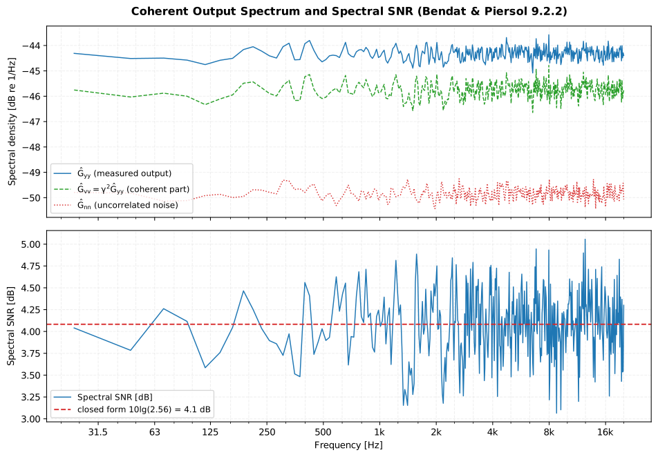

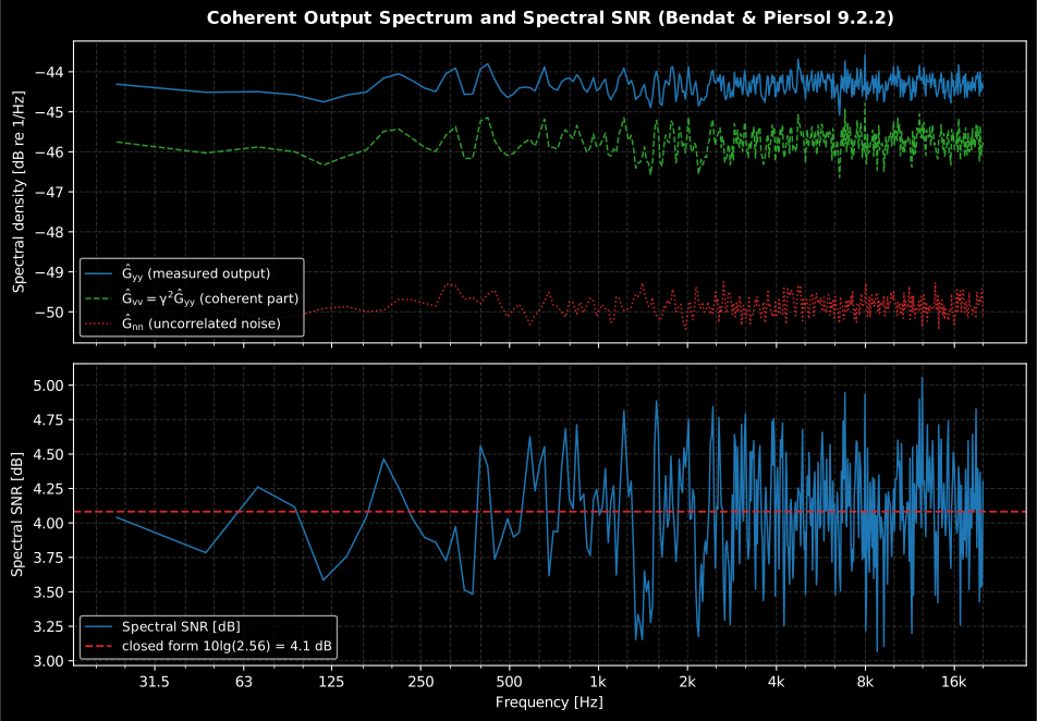
The exact split of the snippet’s model: $G_{vv}={\gamma }^2{G}_{yy}$ explains the output except for the flat noise remainder $G_{nn}$, and the spectral SNR scatters around its closed form $10{\log }_{10}(0.64/0.25)=4.1$ dB at every frequency.

Show the code for this figure

import matplotlib.pyplot as plt
import numpy as np
from phonometry import coherent_output_spectrum, noise_signal

fs = 48000.0
x = noise_signal(fs, 8.0, color="white", seed=1)
noise = noise_signal(fs, 8.0, color="white", rms=0.5, seed=2)
y = 0.8 * x + noise                      # SNR = 0.64/0.25 per band

res = coherent_output_spectrum(x, y, fs, nperseg=2048)

# One line — the three spectra and the SNR panel:
res.plot()
plt.show()

# By hand, from the fields the result carries:
band = (res.frequencies >= 20) & (res.frequencies <= 20000)
freqs = res.frequencies[band]
fig, (ax_g, ax_s) = plt.subplots(2, 1, sharex=True)
for values, style, label in ((res.output_psd, "-", "Gyy (measured)"),
                             (res.coherent_psd, "--", "Gvv (coherent)"),
                             (res.noise_psd, ":", "Gnn (noise)")):
    ax_g.semilogx(freqs, 10 * np.log10(values[band]), style, label=label)
ax_g.set_ylabel("Spectral density [dB re 1/Hz]")
ax_s.semilogx(freqs, res.snr_db[band], label="Spectral SNR [dB]")
ax_s.axhline(10 * np.log10(0.64 / 0.25), color="r", linestyle="--",
             label="closed form 4.1 dB")
ax_s.set(xlabel="Frequency [Hz]", ylabel="SNR [dB]")
for ax in (ax_g, ax_s):
    ax.legend()
plt.show()

The coherence_bias field reports the small positive bias of the coherence estimate, $b[{\hat{\gamma }}^2]\approx (1-{\gamma }^2{)}^2/n_d$ (Eq. 9.75), negligible once $n_d$ reaches a few hundred, and another reason to average generously before trusting a low coherence.

Two channels in practice

Sections 2 and 3 both start from a pair of records, and everything they report is only as good as the pair. Two halves: how to acquire it, and how to read a coherence that comes back below one.

Acquisition. Use one interface with simultaneously sampled inputs, or measure the inter-channel skew and remove it. A converter that sequences its channels puts a fixed skew straight into the cross-spectrum phase and therefore into every group delay read off it: one sample of skew at 48 kHz is 20.8 µs, which is 15° of phase at 2 kHz and a flat 20.8 µs error on any delay estimate. Set both gains before the run and do not touch them, because the coherent output split of section 3 assumes the two channels share a fixed scale. Validate the pair once with a zero-baseline run: feed both channels the same signal — the generator split into both inputs, or the two microphones side by side — and confirm that the measured delay is a small fraction of a sample and the coherence is unity across the band. That one run separates a chain problem from a physics problem for every measurement afterwards.

Reading a coherence below one. It is not automatically an SNR problem, and Bendat & Piersol name five causes with different fixes:

What you see	The cause	The fix
Coherence flat across the band, consistent with ${\gamma }^2=\mathrm{SNR}/(1+\mathrm{SNR})$	uncorrelated noise at either sensor — the modelled case of section 3	average more, raise the level, get closer
Coherence falling progressively with frequency, worse as the record is segmented shorter	a bulk propagation delay comparable with the segment length	align the records first, or raise nperseg well above the delay — see Correlation and delay
Sharp dips exactly at the resonances	resolution bias: the analysis bandwidth smears the peak differently in the two channels	lengthen the segment; the ${\epsilon }_b$ formula of section 1 says by how much
Low at the harmonics of a strong tone while broadband coherence stays high	non-linearity, a rattle or a clipped channel	fix the path, or work below the level at which it appears
Low over a band with no obvious structure	a second, uncorrelated source is also driving the output	the MISO page: one input cannot explain two sources

Two closing cautions. The coherence estimate is biased high by $(1-{\gamma }^2{)}^2/n_d$, so a low coherence read from a handful of averages is even lower than it looks. And read the other way, a coherence near one is the acceptance criterion that makes the whole estimate reportable: quote it band by band beside the transfer function, because the bands where it falls are exactly the bands where the numbers above it mean nothing.

4. Fractional-octave smoothing

fractional_octave_smoothing averages a spectrum over a rectangular window of constant relative width: 1/n octave, $[f\cdot 2^{-1/2n},f\cdot 2^{+1/2n}]$ around each frequency. This is the constant-percentage resolution bandwidth that Bendat & Piersol recommend for the spectra of resonant systems (Section 8.5.3), and the de facto standard for presenting loudspeaker and room responses. The average is always computed on power (amplitudes are squared first, dB levels converted and back), so band power is conserved rather than amplitude, and a flat spectrum passes through exactly unchanged.

The three domain= values name what the ordinate you hand it is, because the averaging is always done on power and the conversion back has to know where it started: a density or a power spectrum ("power", the default), a linear magnitude such as a frequency-response $|H|$ ("amplitude", squared first), or a curve already in decibels ("db", converted and converted back).

from phonometry import fractional_octave_smoothing

freqs = res.frequencies                    # from the section 1 estimate
smooth_psd = fractional_octave_smoothing(freqs, res.psd, 3.0)
magnitude = np.sqrt(res.psd)               # any linear |H| would do here
smooth_mag = fractional_octave_smoothing(freqs, magnitude, 6.0,
                                         domain="amplitude")  # an FRF |H|
levels = 10.0 * np.log10(res.psd)          # any dB curve would do here
smooth_db = fractional_octave_smoothing(freqs, levels, 3.0, domain="db")

A single spectral line with PSD ordinate $P$ (units²/Hz) in a bin of width $\Delta f$ smooths to the closed-form level $P\Delta f/(f_0(2^{1/2n}-2^{-1/2n}))$ over one kernel width, the oracle pinned in the tests.

A smoothed density is still a density

Smoothing changes the resolution of the estimate, never its units. The output of fractional_octave_smoothing is a density in units²/Hz, exactly as the input was — flat white noise smooths to the same flat density — whereas the one-third-octave band levels of that same white noise rise 3 dB per band. Overlay a smoothed PSD on a filter-bank spectrum without converting and the two disagree by 20 to 30 dB, and neither is wrong.

The conversion is one term. A fractional-octave band of centre frequency $f_c$ has bandwidth $B_n=f_c(2^{1/2n}-2^{-1/2n})$, that is $0.2316f_c$ in one third of an octave and $0.7071f_c$ in a full octave, so

$$L_{\text{band}}=10{\log }_{10}\left(\frac{G(f_c)B_n}{p_0^2}\right),$$

which at 1 kHz in one-third octave adds $10{\log }_{10}(0.2316\times 1000)=23.65$ dB to the density level, and 3 dB more for every octave upward. Summing the PSD bins across the band and multiplying by the bin spacing is the exact form; the expression above is its flat-within-the-band approximation.

Which presentation belongs where: the smoothed density for comparing loudspeaker and room magnitude responses, where the eye wants a curve at constant relative resolution; the band level for anything that faces a criterion, or that has to agree with octave_filter and OctaveFilterBank — see Levels.

5. Colored-noise generators

noise_signal produces Gaussian noise whose PSD follows $G_{xx}(f)\propto f^{\alpha }$ exactly in expectation: seeded white noise is shaped in the frequency domain by the exact magnitude response $(f/f_{\text{ref}}{)}^{\alpha /2}$ bin by bin (a zero-phase filter applied circularly), so a measured slope deviates from the power law only by the random error of the spectral estimate, not by the piecewise or few-pole pink approximations whose slope ripples by fractions of a dB. The record is zero-mean and rescaled to the requested RMS exactly, and the same seed reproduces the same record bit for bit.

color	$\alpha$	PSD slope
white	0	0 dB/octave
pink	-1	-3.01 dB/octave
red (Brownian)	-2	-6.02 dB/octave
blue	+1	+3.01 dB/octave
violet	+2	+6.02 dB/octave

from phonometry import noise_signal

pink = noise_signal(48000, 10.0, color="pink", seed=7)     # deterministic
white = noise_signal(48000, 10.0, color="white", rms=0.5, seed=7)

Measured over three decades (20 Hz – 20 kHz) with the estimator of section 1, the regression slope of each color lands within a few thousandths of a dB/octave of the exact value; the conformance suite pins the pink slope at -3.0116 against the exact -3.0103.

Those slopes are density slopes, and they are not what a fractional-octave display of the same signal shows. A band’s width grows in proportion to its centre frequency, so a band level is the density plus $10{\log }_{10}{B}_n$ with $B_n\propto f_c$: every colour reads 3 dB per octave higher in a band display than its density slope suggests. White noise, whose density is flat, therefore rises 3 dB per octave through an octave-band filter bank, and pink noise, at −3 dB/octave, comes out flat — which is why pink is the reference stimulus for room and loudspeaker work, and why an octave-band spectrum of white noise sloping upward is not a bug. Red noise falls 3 dB per octave in a band display and blue rises 6. The same +3 dB per octave applies to any density-versus-band comparison in this library; section 4 above gives the exact conversion, and Levels is where the band side lives.

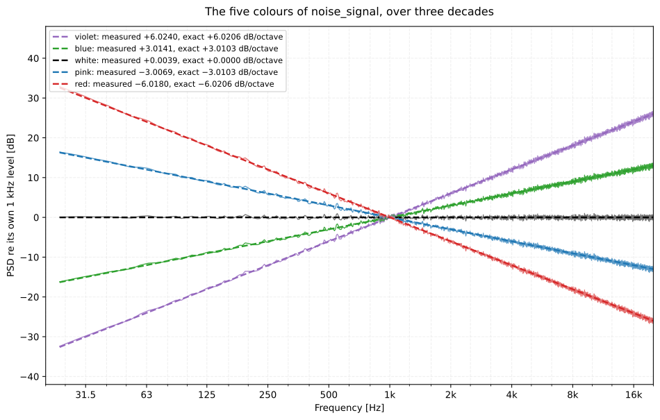
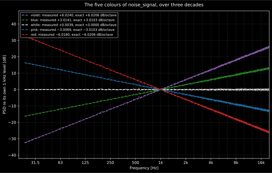
The five generators over three decades, each normalised to its own 1 kHz level so the slopes fan out from one point, with the exact power law dashed underneath. The measured regression slopes land within four thousandths of a decibel per octave of the exact values, and the residual is the random error of the estimator, not of the generator: the same seed reproduces the record bit for bit.

6. Choosing the window

Every estimator on this page accepts any window scipy.signal.get_window knows, but the choice is a quantified trade-off, not a preference. window_metrics computes the figures of merit Harris (1978) tabulated, for any taper and length, sampled DFT-even exactly as the Welch estimators apply it:

• ENBW (equivalent noise bandwidth, in bins): how much wider than one bin the effective analysis bandwidth is. This is the same number the PSD result reports as resolution_bandwidth (ENBW·fs/nperseg in Hz), and it enters directly in the tone/noise trade: a broadband noise floor read from a windowed spectrum sits $10{\log }_{10}(\mathrm{ENBW})$ dB above the true density.
• Coherent gain: the DC gain $\sum w/N$ a bin-centered tone is scaled by.
• Scalloping loss: the worst-case attenuation of a tone that falls midway between two bins (3.92 dB for rectangular, 1.42 dB for Hann).
• Worst-case processing loss: scalloping plus $10{\log }_{10}(\mathrm{ENBW})$, the worst-case reduction in output SNR for tone detection in white noise.
• Highest sidelobe and main-lobe -3 dB width: leakage floor versus resolution.

from phonometry import window_metrics

m = window_metrics("hann", 2048)
print(m.enbw_bins)              # 1.5, exactly
print(m.scalloping_loss_db)     # 1.42 dB
print(m.highest_sidelobe_db)    # -31.5 dB
m.plot()                        # window + spectrum with metrics marked

The closed forms anchor the tests: ENBW is exactly 1 for rectangular, 3/2 for Hann, 1987/1458 for Hamming and 1523/882 for Blackman (DFT-even sampling), and the rectangular scalloping loss is $20{\log }_{10}(N\sin (\pi /2N))$, the Dirichlet kernel evaluated half a bin off center.

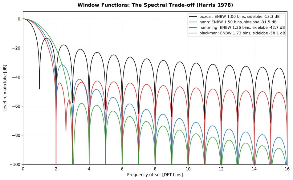
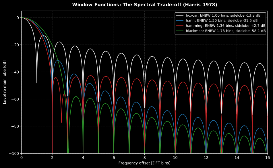
The trade in one picture, and it costs 44.8 dB of leakage floor to buy 0.73 of a bin. Going from rectangular to Blackman drops the highest sidelobe from −13.3 dB to −58.1 dB while the ENBW widens from 1.000 to 1.727 bins and the −3 dB main lobe from 0.886 to 1.644 bins. Hann sits where the module’s default sits: −31.5 dB for 1.500 bins. Read the two axes together — a narrow main lobe separates two tones of similar level, a low sidelobe floor finds a weak tone beside a strong one, and no window does both.

Show the code for this figure

import matplotlib.pyplot as plt
import numpy as np
from phonometry import window_metrics

n, oversample = 1024, 256
fig, ax = plt.subplots(figsize=(10, 6.2))
for name in ("boxcar", "hann", "hamming", "blackman"):
    res = window_metrics(name, n)
    spectrum = np.abs(np.fft.rfft(res.taps, n=n * oversample))
    level = 20.0 * np.log10(spectrum / spectrum[0])
    bins = np.arange(level.size) / oversample
    shown = bins <= 16.0
    ax.plot(bins[shown], level[shown],
            label=(f"{name}: ENBW {res.enbw_bins:.2f} bins, "
                   f"sidelobe {res.highest_sidelobe_db:.1f} dB"))
ax.set_xlim(0.0, 16.0)
ax.set_ylim(-100.0, 5.0)
ax.set_xlabel("Frequency offset [DFT bins]")
ax.set_ylabel("Level re main lobe [dB]")
ax.legend(loc="upper right")
plt.tight_layout()
plt.show()

The Hann default of this module is the balanced choice: fast sidelobe falloff (-18 dB/octave) protects noise spectra from leakage, ENBW 1.5 costs only 1.76 dB against the rectangular window, and its overlap correlation at 50 % keeps nearly all segment information in the effective average count. Reach for a lower-sidelobe taper (Blackman, Kaiser with a high beta) when a weak tone must be found next to a strong one, and accept the wider main lobe; reach for the rectangular window only for self-windowing records (transients that decay inside the segment) or bin-centered synthesis.

7. Multitaper estimation for short records

Welch’s method buys stability with record length: each independent segment adds two degrees of freedom, so a record that only fits a couple of segments leaves an estimate barely better than a periodogram. multitaper_psd implements the alternative of Thomson (1982), as developed by Percival & Walden (1993, Chapter 7): the whole record is multiplied by $K$ orthogonal discrete prolate spheroidal (Slepian) tapers - the sequences that concentrate the most spectral-window energy inside a chosen design band $[-W,W]$ - and the $K$ resulting eigenspectra are averaged:

$${\hat{S}}^{(mt)}(f)=\frac{1}{K}\sum _{k=0}^{K-1}{\hat{S}}_k(f),{\hat{S}}_k(f)=\Delta t|\sum _{t=1}^N{h}_{t,k}{x}_t{e}^{-i2\pi ft\Delta t}{|}^2.$$

Because the tapers are orthogonal the eigenspectra are nearly uncorrelated, so the average carries about $2K$ chi-square degrees of freedom from a single record - the same statistical machinery as the Welch result (random error, chi-square confidence interval), without segmenting. The design parameter is the dimensionless duration-times-half-bandwidth product $p=NW$ (default 4), and for a record of $N_r$ samples at $f_s$ it fixes the half-bandwidth $W=p{f}_s/N_r$ in hertz. $2W$ is the resolution of the estimate (reported as resolution_bandwidth), and only the tapers below the Shannon number $2p$ keep their spectral-window energy inside the design band - their concentrations ${\lambda }_k$ are reported as eigenvalues, and the default taper count is $K=2p-1$, all tapers with near-unity concentration. Larger $p$ admits more tapers (lower variance) at the cost of resolution.

from phonometry import multitaper_psd

res = multitaper_psd(record, fs)                 # p = NW = 4, K = 7, adaptive
print(res.degrees_of_freedom.mean())             # ~2K from one record
print(res.eigenvalues)                           # taper concentrations
res.plot()                                       # density with the CI band

By default the eigenspectra are combined with Thomson’s adaptive weights (P&W Eqs. 368a/370a, iterated to convergence). Each taper’s weight at each frequency balances the local spectrum against the broad-band leakage the taper could carry:

$$b_k(f)=\frac{S(f)}{{\lambda }_{k}S(f)+(1-{\lambda }_k){\sigma }^2\Delta t},{\hat{S}}^{(amt)}(f)=\frac{{\sum }_k{b}_k^2(f){\lambda }_k{\hat{S}}_k(f)}{{\sum }_k{b}_k^2(f){\lambda }_k},$$

so the leakier high-order tapers are downweighted exactly where the spectrum is locally weak, and nothing is lost where it is locally white (for white noise the weights are uniform). The price is bookkept honestly: the equivalent degrees of freedom become frequency dependent, $\nu (f)=2{\left({\sum }_k{d}_k\right)}^2/{\sum }_k{d}_k^2$ with $d_k=b_k^2{\lambda }_k$ (P&W Eq. 370b), and the confidence interval widens wherever leakage protection spent them. adaptive=False selects the plain eigenvalue-weighted average instead.

Calibration matches the Welch estimators exactly: no detrending, 'density' integrates to the signal power, and 'spectrum' reads $A^2/2$ at the peak of a sinusoid of amplitude $A$ (a tone’s power in 'density' scaling spreads over the $2W$ band). The Slepian tapers themselves come from scipy.signal.windows.dpss; their concentrations reproduce the quadruple-precision table of Percival & Walden (Table 382) to machine precision, which is the anchor oracle of the test suite.

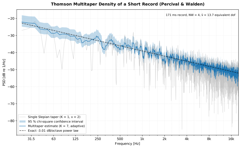
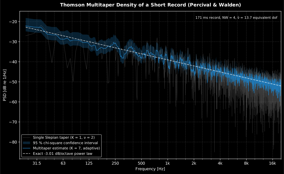
Left, the case the text claims multitaper wins: a 171 ms record. Welch with a 2048-sample segment fits only $n_d=6.7$ effective averages into it, so its confidence band is visibly the wider of the two and its curve the rougher, while the 7-taper adaptive estimate carries 13.7 equivalent degrees of freedom from the same record. Right, the other reason to reach for it: a 60 dB tone over a pink floor. The Hann taper leaves a broader skirt around the tone than the adaptive weights do, and the price is printed on the right-hand axis — the equivalent degrees of freedom fall wherever the weights bought that protection, which is exactly what widens the confidence interval there.

Show the code for this figure

import matplotlib.pyplot as plt
import numpy as np
from phonometry import multitaper_psd, noise_signal

fs = 48000.0
x = noise_signal(fs, 8192 / fs, color="pink", seed=11)   # 171 ms record
single = multitaper_psd(x, fs, n_tapers=1, adaptive=False)
res = multitaper_psd(x, fs)                              # NW = 4, K = 7
band = (res.frequencies >= 20.0) & (res.frequencies <= 20000.0)
freqs = res.frequencies[band]

fig, ax = plt.subplots(figsize=(10, 6))
ax.semilogx(freqs, 10 * np.log10(single.psd[band]), color="gray",
            alpha=0.45, lw=0.7, label="Single Slepian taper (K = 1)")
ax.fill_between(freqs, 10 * np.log10(res.ci_lower[band]),
                10 * np.log10(res.ci_upper[band]), alpha=0.3,
                label="95 % chi-square confidence interval")
ax.semilogx(freqs, 10 * np.log10(res.psd[band]), lw=1.2,
            label="Multitaper estimate (K = 7, adaptive)")
ax.set_xlabel("Frequency [Hz]")
ax.set_ylabel("PSD [dB re 1/Hz]")
ax.legend()
plt.show()

Reach for multitaper_psd when the record is too short to segment (room impulse response tails, transient captures, single machine cycles) or when a high-dynamic-range spectrum needs leakage protection that a Hann-windowed Welch average cannot give; stay with power_spectral_density for long records, where segment averaging is cheaper than $K$ full-length FFTs and the two estimators agree.

Consistency with the frequency-response and intensity estimators

The frequency-response estimators form the same cross-spectra into a transfer function — $H_1=G_{xy}/G_{xx}$, unbiased when the noise is on the output, and $H_2=G_{yy}/G_{yx}$, unbiased when it is on the input — and the two-microphone sound intensity probe forms the imaginary part of $G_{xy}$. Those estimators, transfer_function and coherence, the intensity probe and these estimators all share one Welch core (same taper, overlap policy and detrend-off calibration), so a PSD, a coherence and an $H_1$ computed with the same segment length are mutually consistent bin by bin. The same cross-spectral matrix underlies multiple and partial coherence, which extends the ordinary coherence to several correlated inputs and one output.

What this guide covers

• Covered

  Bendat & Piersol’s Welch estimators (Random Data, 4th ed., 2010, Sections 5.2, 8.5, 9.1-9.2 and 11.5): power_spectral_density and cross_spectral_density with the effective number of averages, chi-square confidence intervals and the resolution-bias error; the coherent output spectrum and spectral SNR; the Harris (1978) window figures of merit of window_metrics; and the Thomson (1982) multitaper estimator of multitaper_psd, following Percival & Walden’s Chapters 7-8. fractional_octave_smoothing and noise_signal complete the toolbox.

• Not covered

  The frequency-response estimators transfer_function and coherence, and the sound-intensity probe, share this page’s Welch core but are documented on the electroacoustics and sound intensity pages, not here. So is multiple and partial coherence, on the MISO coherence page. This page implements Bendat & Piersol’s textbook estimators, not a certification standard, so it carries no clause numbers or compliance limits to check against.

See also

• Data qualification: the stationarity every chi-square interval on this page assumes.
• Calibration and dBFS: where the factor that turns this page’s densities into Pa²/Hz comes from.
• MISO coherence: the same cross-spectral matrix with several correlated inputs.
• Time-frequency analysis: the same Welch segmentation displayed instead of averaged.
• Levels: the band-level side of the density/band conversion of section 4.
• API reference: signals.spectra, signals.windows and signals.multitaper.
• Theory: Frequency Resolution vs FFT Bin Spacing: why the bin spacing of an FFT is not the resolution of the estimate, and what the window does to both.

References

• Bendat, J. S., & Piersol, A. G. (2010). Random data: Analysis and measurement procedures (4th ed.). Wiley. https://doi.org/10.1002/9781118032428Sections 5.2 and 8.5 (autospectra and their random/bias errors, chi-square intervals), 9.1-9.2 (cross-spectra, coherent output spectrum and their errors) and 11.5 (Welch processing, tapering and overlap). ISBN 978-0-470-24877-5.
• Harris, F. J. (1978). On the use of windows for harmonic analysis with the discrete Fourier transform. Proceedings of the IEEE, 66(1), 51-83. https://doi.org/10.1109/PROC.1978.10837The window figures of merit (Table 1): equivalent noise bandwidth, coherent gain, scalloping loss, worst-case processing loss, highest sidelobe level and main-lobe width, computed by window_metrics for any scipy taper.
• Percival, D. B., & Walden, A. T. (1993). Spectral analysis for physical applications: Multitaper and conventional univariate techniques. Cambridge University Press. https://doi.org/10.1017/CBO9780511622762Chapter 7 (multitaper estimation: eigenspectra, adaptive weighting, equivalent degrees of freedom) and Chapter 8 (computing the Slepian sequences); the Table 382 eigenvalues anchor the taper oracle in the test suite. ISBN 978-0-521-43541-3.
• Thomson, D. J. (1982). Spectrum estimation and harmonic analysis. Proceedings of the IEEE, 70(9), 1055-1096. https://doi.org/10.1109/PROC.1982.12433The multitaper method: Slepian tapers, eigenspectra and the adaptive weights implemented by multitaper_psd.
• Welch, P. D. (1967). The use of fast Fourier transform for the estimation of power spectra: A method based on time averaging over short, modified periodograms. IEEE Transactions on Audio and Electroacoustics, 15(2), 70-73. https://doi.org/10.1109/TAU.1967.1161901The overlapped-segment variance formula behind the effective number of averages (Bendat & Piersol Section 11.5.2.2, Ref. 11).