Sound pressure tells you how loud a point is; sound intensity tells you where the energy is going. It is the acoustic power flux (W/m²), a signed vector quantity, which is why intensity probes can localize sources, separate them from background noise and measure sound power in situ (ISO 9614) where a pressure measurement alone cannot.
The two-microphone principle (IEC 61043)
Section titled “The two-microphone principle (IEC 61043)”A p-p probe holds two matched microphones a small distance apart. The pressure at the probe center is their mean, and the particle velocity comes from the pressure gradient (Euler’s equation, finite-difference form):
In practice the estimator works in the frequency domain through the cross-spectrum of the two channels (the standard’s equivalent form):
Everything on this page is then read as a level. The sound intensity level
is with : the
level is of the magnitude, and the direction is carried separately, which is
what total_direction reports as . The two references were chosen to
line up: in a plane progressive wave, where , the pressure and
intensity levels agree to within dB at
ordinary air conditions (IEC 61043 clause 5). That is why the left panel of the
figure below shows two curves lying on top of each other, and why the
pressure-intensity index has a floor near 0.14 dB rather than 0. Everything a
field measurement shows above that floor is either a genuinely reactive or
noise-contaminated field, or the instrument’s own phase error.
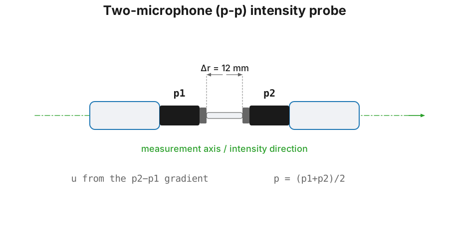
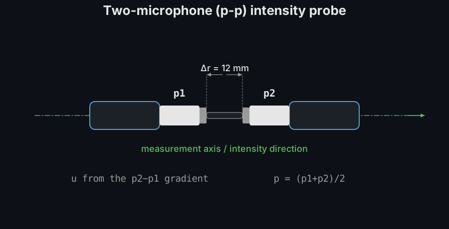
The probe itself is small enough to draw at true scale.
plot_pp_probe_geometry puts the classic 12 mm solid spacer between the two
face-to-face capsules, and a computed IntensityResult that retained its
spacing redraws its own probe with res.plot_geometry().
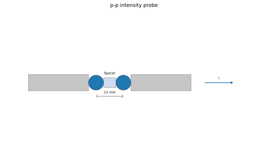
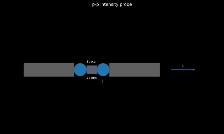
The finite difference at true scale: two half-inch capsules face to face across 12 mm of solid spacer, and that is both the sensitivity of the gradient estimate and the origin of the high-frequency error.
Show the code for this figure
import matplotlib.pyplot as pltfrom phonometry import emission
# The classic 12 mm solid spacer between two half-inch microphones.emission.plot_pp_probe_geometry()plt.show()
# A computed IntensityResult retains its spacing:#   res = emission.sound_intensity(p1, p2, fs, spacing=0.012)#   res.plot_geometry()
The measurement itself is two synchronous channels: p1 and p2 are the
calibrated pressures of the two capsules in pascals, p1 the one nearer the
source, acquired on the same analyser at the same sampling rate with the probe
axis normal to the measurement surface.
import numpy as npfrom phonometry import emission
fs = 48000rng = np.random.default_rng(0)# The two probe-microphone pressures in Pa, p1 closest to the source.#   In a real measurement these are your two calibrated probe recordings;#   synthesized here (p2 = p1 delayed one sample) so the guide runs.p1 = 0.02 * rng.standard_normal(fs)p2 = np.concatenate(([0.0], p1[:-1]))   # p2 = p1 delayed one sample
res = emission.sound_intensity(p1, p2, fs, spacing=0.012, fraction=3,                      limits=[100, 2500])print(res.total_intensity_level, res.total_direction)      # LI [dB], ±1print(res.frequencies, res.intensity_level)                  # per bandres.plot()   # Lp vs LI per band + the pressure-intensity index (needs matplotlib)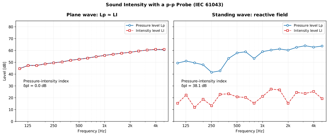
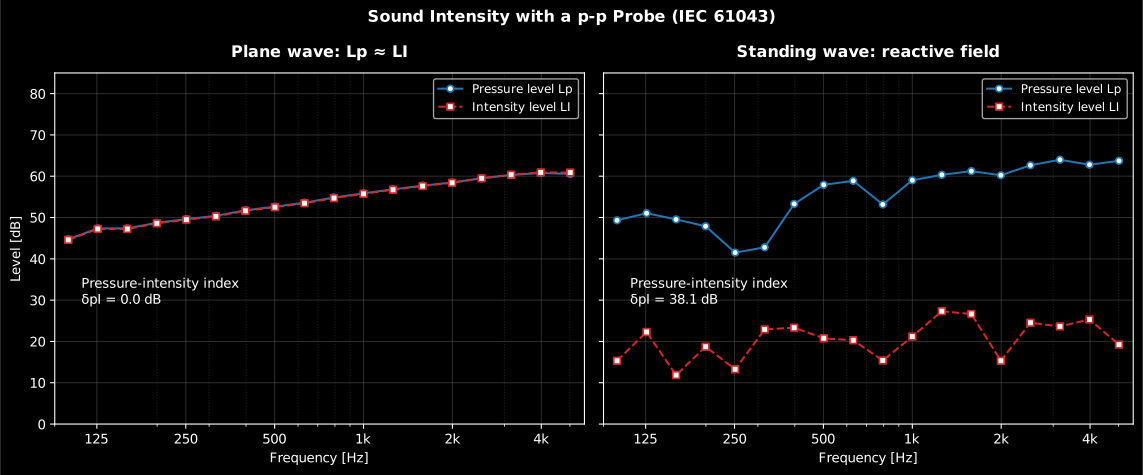
Left: in a plane progressive wave all pressure is transported, so . Right: a standing wave carries (almost) no net energy, so the pressure is high but the intensity collapses. The gap is the pressure-intensity index, the fundamental quality indicator of every intensity measurement.
Show the code for this figure
import matplotlib.pyplot as pltimport numpy as npfrom scipy import signalfrom phonometry import emission
fs, dr, c = 48000, 0.012, 343.0n = int(fs * 4.0)
# Broadband noise, band-limited to 80 Hz - 6 kHz and scaled to about 70 dB SPL.rng = np.random.default_rng(2026)noise = signal.sosfilt(    signal.butter(4, [80.0, 6000.0], btype="bandpass", fs=fs, output="sos"),    rng.standard_normal(n),)noise *= 0.063 / np.std(noise)spectrum = np.fft.rfft(noise)freqs = np.fft.rfftfreq(n, 1 / fs)
# Left: a plane progressive wave. Microphone 2 sees the wave dr/c = 35 us later,# applied as a phase shift rather than as a whole number of samples.plane = emission.sound_intensity(    noise, np.fft.irfft(spectrum * np.exp(-2j * np.pi * freqs * dr / c), n),    fs, spacing=dr, fraction=3, limits=[100.0, 5000.0],)
# Right: a standing wave, two equal counter-propagating waves, with the probe# centred at x0 = 0.30 m from the rigid termination.k, x0 = 2 * np.pi * freqs / c, 0.30def at(pos):    return np.fft.irfft(spectrum * 2.0 * np.cos(k * pos), n)standing = emission.sound_intensity(at(x0 - dr / 2), at(x0 + dr / 2),                                    fs, spacing=dr, fraction=3,                                    limits=[100.0, 5000.0])
fig, (axl, axr) = plt.subplots(1, 2, figsize=(12, 5), sharey=True)plane.plot(ax=axl)standing.plot(ax=axr)plt.show()
The same contrast plays out dynamically below: the pressure and velocity phasors of a progressive and a standing wave, with the instantaneous intensity averaging to a net flow in one case and to zero in the other.
A two-microphone p-p probe with rotating pressure and velocity phasors; the instantaneous intensity arrow flips while its running average settles to a net flow for the progressive wave and to zero for the standing wave.
A two-microphone p-p probe with rotating pressure and velocity phasors; the instantaneous intensity arrow flips while its running average settles to a net flow for the progressive wave and to zero for the standing wave.
Knowing when to trust the number
Section titled “Knowing when to trust the number”Two physical limits bound every p-p measurement, and the result object carries both:
- High frequency: the finite-difference gradient underestimates by
, verified in CI against IEC 61043 Table 3.
IntensityResult.bias_correctionprovides the factor andmax_valid_frequency(; 2.9 kHz for a 12 mm spacer) the practical ceiling. Larger spacers reach lower frequencies, smaller ones higher. - Reactive fields: when
pressure_intensity_index( in ISO 9614-1) approaches the probe’s residual index , phase errors dominate.
Three symbols recur from here on, and they are derived in The margin over the residual index below: is the residual pressure-intensity index, the phase-error floor of the probe-spacer-analyser chain; is the bias factor the grade allows (10 dB engineering, 7 dB survey); and is the dynamic capability, the largest field index the instrument can afford at that grade.
Before any of that, ISO 9614-1 asks a question about the field rather than the surface: is it steady enough to be scanned at all? In the initial test (clause 8.2) one typical position is picked on an initial measurement surface and the normal intensity is sampled there times with a short averaging time (Note 9 suggests , and, for periodic signals, 8 s to 12 s per sample or any whole number of cycles). , the temporal variability indicator, is the coefficient of variation of those samples (equations (A.1)–(A.2)), so it is zero for a perfectly steady field and grows as the extraneous intensity wanders. Table B.3 asks for action code (e) when exceeds 0.6: reduce the variability, measure during quieter periods, or lengthen the averaging time at each position. Annex B also has it evaluated immediately before and after the measurement on any one surface (B.1.4).
from phonometry import emission
# The M short-time samples of the normal intensity at one fixed position (W/m²).samples = [1.20e-5, 0.94e-5, 1.51e-5, 1.08e-5, 1.33e-5,           1.02e-5, 1.44e-5, 1.17e-5, 0.88e-5, 1.29e-5]
f1 = emission.temporal_variability_indicator(samples)print(round(f1, 3))                          # 0.177, a steady field
# Or carried on the surface result alongside F2/F3/F4, by handing the same# samples to field_indicators together with the per-position scan below:fi = emission.field_indicators([74.1, 73.8, 74.5, 73.2],                               [1.2e-5, 1.0e-5, 1.4e-5, 0.9e-5],                               temporal_intensity=samples)print(fi.field_is_stationary())              # True (Table B.3 limit 0.6)
Over a measurement surface, the remaining ISO 9614-1 Annex A field indicators grade the scan itself. , the surface pressure-intensity indicator, is the surface pressure level minus the level of the mean magnitude of the normal intensity: the larger it is, the closer the measurement sits to the probe’s phase-error floor. , the negative partial power indicator, is the same difference taken with the signed mean intensity: reveals power flowing inward through parts of the surface. , the field non-uniformity indicator, is the normalised spread of the per-position intensities: the larger it is, the more measurement positions the surface needs.
is the one that turns into a number of positions, through criterion 2 of Annex B, (Eq. B.2). The factor is not a constant: Table B.2 makes it depend on the band and on the grade being claimed: about 11 at low frequency rising to 29 in the mid band for engineering grade, and 19 rising to 57 for precision, with 8 for the A-weighted survey case. So the same field non-uniformity asks for roughly twice as many positions at grade 1 as at grade 2. Worked: in the 1 kHz band needs , so at least 8 positions at engineering grade and at least 15 at precision; and when one position count is used for every band, the standard applies the criterion at the band with the largest .
is also directly reportable, which is what makes it worth computing even when the count is already fixed: the 95 % confidence interval on a band level is (Eq. B.3), so over 10 positions carries +1.2 dB / −1.7 dB. A band that fails criterion 2 may still be recorded, but only accompanied by that interval.
Together with the dynamic-capability criterion the indicators are available directly:
import numpy as npfrom phonometry import emission
# Per-position measurements over the ISO 9614-1 measurement surfacepressure_levels = np.array([74.1, 73.8, 74.5, 73.2])       # Lp per position (dB)normal_intensity = np.array([1.2e-5, 1.0e-5, 1.4e-5, 0.9e-5])  # signed In per position (W/m²)
fi = emission.field_indicators(pressure_levels, normal_intensity)print(round(fi.f2, 2), round(fi.f3, 2), round(fi.f4, 3))   # 3.41 3.41 0.197ld = emission.dynamic_capability_index(18.0)   # δpI0 = 18 dB → Ld = δpI0 − Kprint(ld, ld > fi.f2)                                      # 8.0 True (criterion 1)
With 2D (positions, bands) arrays and the band centres the indicators come
back per band, and the result is plottable in one line, the form in which
the criteria are actually checked (each band passes or fails on its own):
# The scan the figure below is drawn from: ten positions over six octave# bands, a nearly uniform surface pressure, and a normal intensity per band# that turns the field reactive towards low frequency, with two inward-flowing# positions in the 125 Hz band (rescaled so the band mean keeps its target).freqs = np.array([125.0, 250.0, 500.0, 1000.0, 2000.0, 4000.0])delta_pi = np.array([10.5, 8.5, 6.0, 4.5, 3.5, 3.0])   # target Lp − L|In|rng = np.random.default_rng(9614)lp_bands = 78.0 + rng.normal(0.0, 0.4, (10, freqs.size))i_mean = 10.0 ** ((78.0 - delta_pi) / 10.0) * 1.0e-12in_bands = i_mean[None, :] * (1.0 + rng.normal(0.0, 0.18, (10, freqs.size)))in_bands[:2, 0] = -0.35 * i_mean[0]in_bands[2:, 0] *= (10.0 * i_mean[0] - in_bands[:2, 0].sum()) / in_bands[2:, 0].sum()
fi = emission.field_indicators(lp_bands, in_bands, freqs)   # (positions, bands)fi.plot(dynamic_capability=ld)   # F2/F3 per band vs Ld, F4 on a twin axis (needs matplotlib)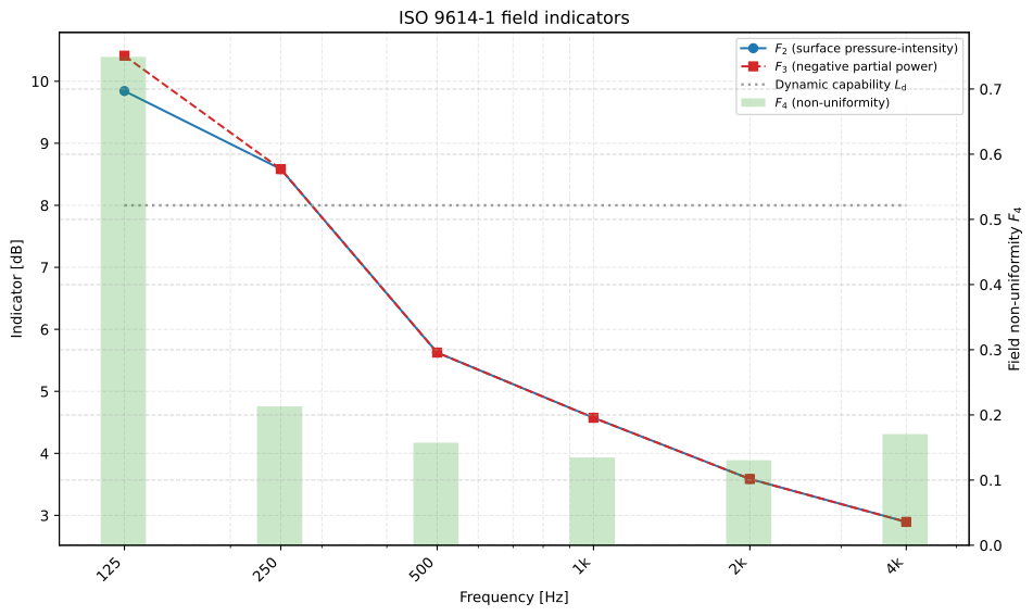
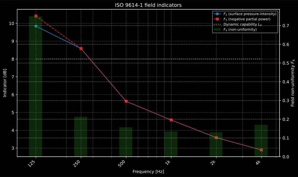
climbs towards low frequency as the field turns reactive, and at 125 Hz it crosses the instrument’s dynamic capability : that band fails criterion 1, and no averaging will fix it. It calls for a larger spacer, a different surface or a quieter room. rising above in the same band reveals inward-flowing (negative) partial intensity, and the bars set the number of positions the surface needs (criterion 2, ).
Show the code for this figure
import matplotlib.pyplot as pltimport numpy as npfrom phonometry import emission
# A 10-position discrete-point scan over six octave bands: the surface# pressure is nearly uniform, and the normal intensity per band is set so the# field turns reactive towards low frequency, with two inward-flowing# positions in the 125 Hz band (rescaled so the band mean keeps its target).freqs = np.array([125.0, 250.0, 500.0, 1000.0, 2000.0, 4000.0])delta_pi = np.array([10.5, 8.5, 6.0, 4.5, 3.5, 3.0])   # target Lp − L|In|rng = np.random.default_rng(9614)lp_bands = 78.0 + rng.normal(0.0, 0.4, (10, freqs.size))i_mean = 10.0 ** ((78.0 - delta_pi) / 10.0) * 1.0e-12in_bands = i_mean[None, :] * (1.0 + rng.normal(0.0, 0.18, (10, freqs.size)))in_bands[:2, 0] = -0.35 * i_mean[0]in_bands[2:, 0] *= (10.0 * i_mean[0] - in_bands[:2, 0].sum()) / in_bands[2:, 0].sum()
fi = emission.field_indicators(lp_bands, in_bands, freqs)ld = emission.dynamic_capability_index(18.0)   # δpI0 = 18 dB, K = 10 dB
# One line — F2/F3 per band against Ld, with F4 on a twin axis:fi.plot(dynamic_capability=ld)plt.show()
# By hand, from the per-band fields the result carries — mirroring what# FieldIndicators.plot() draws (Ld step line, merged twin-axis legend):fig, ax = plt.subplots()ax.plot(fi.frequencies, fi.f2, "o-", label="F2 (surface pressure-intensity)")ax.plot(fi.frequencies, fi.f3, "s--", label="F3 (negative partial power)")ax.plot(fi.frequencies, np.full(fi.frequencies.size, ld), ":", drawstyle="steps-mid", label="Dynamic capability Ld")ax.set_xlabel("Frequency [Hz]")ax.set_ylabel("Indicator [dB]")twin = ax.twinx()twin.bar(fi.frequencies, fi.f4, width=fi.frequencies * 0.2, alpha=0.25, color="#2ca02c", label="F4 (non-uniformity)")twin.set_ylabel("Field non-uniformity F4")lines, labels = ax.get_legend_handles_labels()tlines, tlabels = twin.get_legend_handles_labels()ax.legend(lines + tlines, labels + tlabels)plt.show()A p-p probe traces the serpentine scan over the top face of the measurement box while the normal-intensity arrows appear behind it, and the partial powers of the five faces accumulate into the sound power level L_W.
A p-p probe traces the serpentine scan over the top face of the measurement box while the normal-intensity arrows appear behind it, and the partial powers of the five faces accumulate into the sound power level L_W.
The margin over the residual index
Section titled “The margin over the residual index”The two channels of any real probe and analyzer are never perfectly phase matched. Feed both channels the same signal (the residual-intensity test of IEC 61043): the true intensity is exactly zero, yet the mismatch reports a small false intensity. The gap between the pressure level and that false intensity level is the residual pressure-intensity index , the instrument’s phase-error floor expressed as an index; IEC 61043 grades probes and processors (class 1 / class 2) chiefly by it.
In the field, the measured index says how far the pressure level stands above the level of the net flow, and the systematic error of the intensity estimate is bounded by the margin between the two indices:
A 10 dB margin keeps the bias within about 0.5 dB and a 7 dB margin within about 1 dB; these are precisely the bias factors of ISO 9614, and the dynamic capability is the largest field index the instrument can afford at a given grade. Read it as a budget: every decibel the field’s rises spends a decibel of margin, and when reaches the reading is pure phase error, of either sign. This is why the pressure-intensity index, not the microphone quality, gates the achievable accuracy of every intensity measurement.
Measuring the residual index, and checking the probe
Section titled “Measuring the residual index, and checking the probe”is the number every criterion on this page and the whole scanning page rests on, and the library does not compute it: it is measured, once per probe-spacer-analyser chain, on a bench.
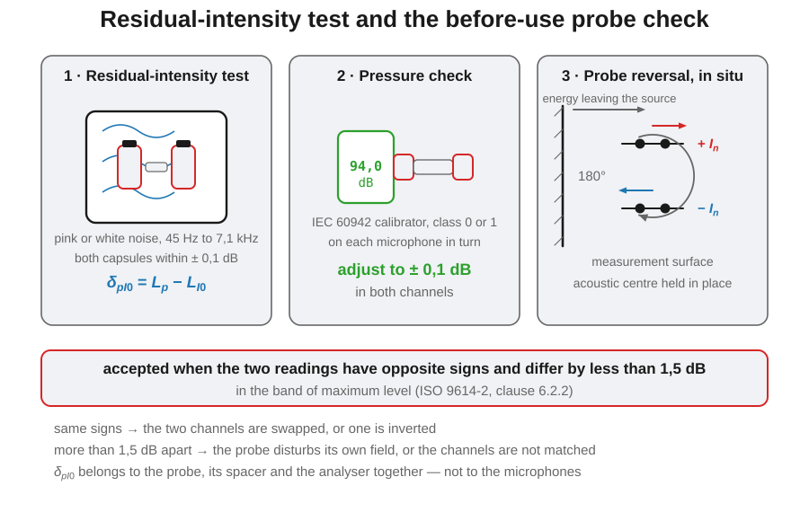
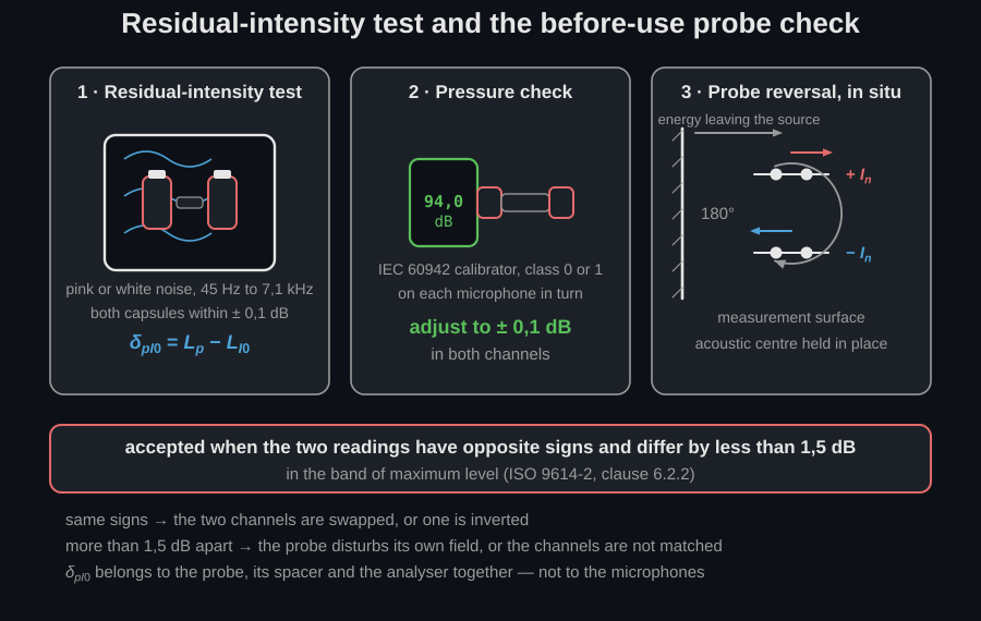
The residual-intensity test (IEC 61043 clause 10.2). The testing device is a small coupler that presents the same sound field to both capsules over the whole or part of 45 Hz to 7,1 kHz, driven with pink or white noise, and applying the pressure to the two microphones at the same level within ±0,1 dB at least from 45 Hz to 1 kHz, with a bounded inter-port phase difference. Because the true intensity in that field is exactly zero, whatever the instrument indicates is its own phase error, and is read band by band as the pressure level minus that indicated intensity level. Two consequences follow from what is in the coupler: the index belongs to the probe, the fitted spacer and the analyser together, so it must be re-measured whenever the spacer changes; and it is a property of the chain, not a specification of the microphones.
Before every series (clause 14). Let the instrument warm up as the manufacturer says. In sound-pressure mode, apply a sound calibrator to the two microphones, in turn or simultaneously, and adjust to the correct indication within ±0,1 dB in both channels: ISO 9614-2 clause 6.2.1 asks for a class 0 or class 1 IEC 60942 calibrator here. Then apply the residual-intensity device again and confirm that still meets the class requirement over the range the device covers, with the manufacturer’s phase compensation applied and, preferably, at a level close to the level of use.
In situ (ISO 9614-2 clause 6.2.2): the probe-reversal test. This is the one check that needs no bench and catches the error no bench can see. Place the probe on the measurement surface, axis normal, at a position where the intensity exceeds the surface mean; record in every band. Rotate the probe 180° about an axis normal to the measurement axis, keeping the acoustic centre in the same place, which in practice means mounting it on a stand rather than holding it, and measure again. For the measurement system to be acceptable, in the band of maximum level the two values of must have opposite signs and the two intensity levels must differ by less than 1,5 dB. Read the two failure modes as diagnoses: identical signs mean the channels are swapped or one is inverted, and a difference above 1,5 dB means the probe is disturbing its own field or the two channels are not matched. Clause 10.5 c) makes the result part of the test report.
That sign is worth reading in normal use too, not only in the check. A negative net intensity over part of an enclosing surface means more power entering that patch than leaving it: entirely normal on the shadow side of a machine standing beside a louder one, and completely meaningless if the channels are swapped.
Grading the instrument: IEC 61043 Table 2
Section titled “Grading the instrument: IEC 61043 Table 2”is not just a number to subtract from; it is what IEC 61043 grades the hardware by. Table 2 of the standard sets a minimum in every one-third-octave band from 50 Hz to 6.3 kHz, separately for a probe, a processor and a complete instrument, in class 1 and class 2, printed for the nominal 25 mm microphone separation. Note 1 rescales the whole table for any other spacer by with in millimetres, which is the same 3 dB per doubling the previous section arrived at from the physics.
verify_intensity_class compares a measured spectrum
against both
masks band by band and returns an IntensityInstrumentComplianceResult holding
the class the chain actually meets: the loosest class every band clears, or
None when some band clears neither.
from phonometry import emission
# The band centres Table 2 is defined on, and the measured residual index of# the chain: one value per band, taken with the spacer that will be fitted in# the field. Replace the placeholder with your own residual-intensity test.freqs, _, _ = emission.residual_index_limits("instrument", spacing=0.012)measured_delta_pi0 = [11.0, 11.9, 11.2, 10.0, 13.2, 15.9, 17.0, 18.0,                      19.0, 20.0, 21.0, 22.0, 23.0, 24.0, 24.0, 24.0,                      24.0, 24.0, 24.0, 24.0, 24.0, 24.0]   # dB, 22 bands
res = emission.verify_intensity_class(measured_delta_pi0, freqs,                                      device="instrument", spacing=0.012)print(res.overall_class)          # 2: one band misses the class 1 minimumprint(res.binding_margin())       # smallest per-band margin to that class [dB]print(res.failing_bands(1))       # the band centres that cost it class 1 [Hz]res.plot()                        # measured δpI0 over the two Table 2 masksres.report("verification.pdf")    # one-page verification fiche (PDF)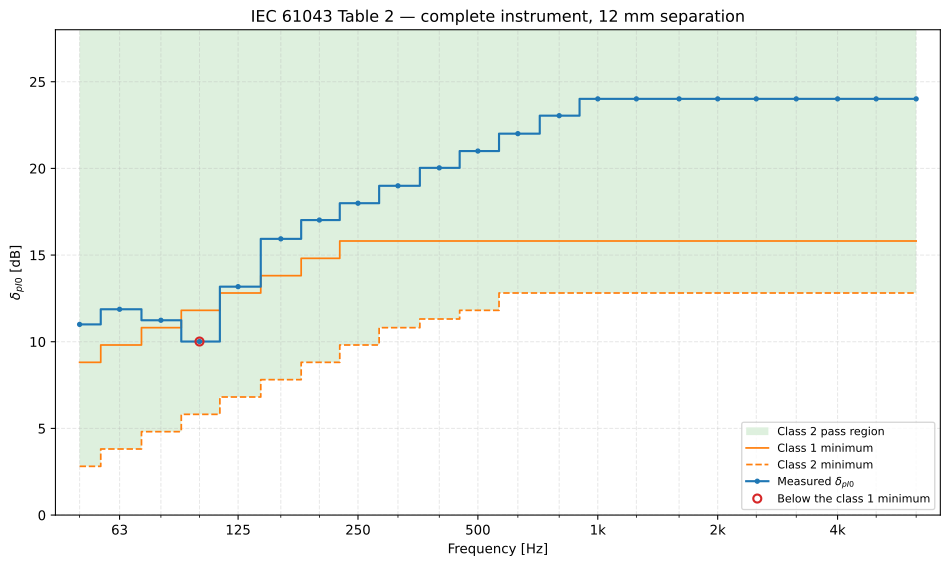
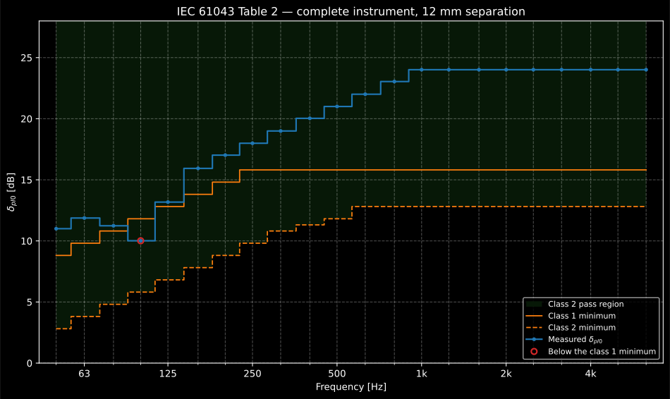
Both Table 2 masks come down by for the 12 mm spacer. The measured index climbs 10 dB per decade at low frequency, parallel to the requirement, because a channel phase mismatch that is constant in degrees buys exactly that slope; it flattens above 1 kHz where the mismatch of a real chain starts growing with frequency instead. A vent resonance around 100 Hz costs 4 dB and drops that one band below the class 1 minimum, so the whole chain is graded class 2.
Show the code for this figure
import matplotlib.pyplot as pltimport numpy as npfrom phonometry import emission
# A complete instrument with the common 12 mm spacer. The measured index is# modelled from the physics behind Table 2: a residual phase mismatch φs reads# as δpI0 = 10 lg(kd/φs), so a mismatch that is constant in degrees already# climbs 10 dB per decade, and above 1 kHz the mismatch of a real chain grows# with frequency, so the index levels off.spacing = 0.012freqs, _, _ = emission.residual_index_limits("instrument", spacing=spacing)phase_mismatch = 0.05 * np.maximum(1.0, freqs / 1000.0)          # degreesmeasured = emission.residual_index_from_phase_mismatch(phase_mismatch, freqs,                                                        spacing)measured = measured - 4.0 * np.exp(-((np.log(freqs / 100.0) / 0.25) ** 2))
res = emission.verify_intensity_class(measured, freqs, spacing=spacing)res.plot()plt.show()
Two companion rules of the standard come with it. Clause 6.1 fixes the
frequency range a class attests: 45 Hz to 7.1 kHz in one-third octaves, which
class 1 requires and class 2 may also use, or 45 Hz to 5.6 kHz in octaves,
which is offered to class 2 as an alternative. A verdict computed over fewer
bands is flagged range_limited so it cannot be read as a full-range claim.
The Spanish translation UNE-EN 61043:1999 records only the octave alternative
for class 2 and drops the one-third-octave one; the library follows the
EN/IEC text (see the
errata registry). Clause 8 combines separately supplied components:
instrument_class_from_components(probe_class, processor_class) returns 1
only when both are class 1, and 2 for every other pairing.
The example fiche is regenerated with make reports and kept rendered in the
repository; click the preview to open the PDF.
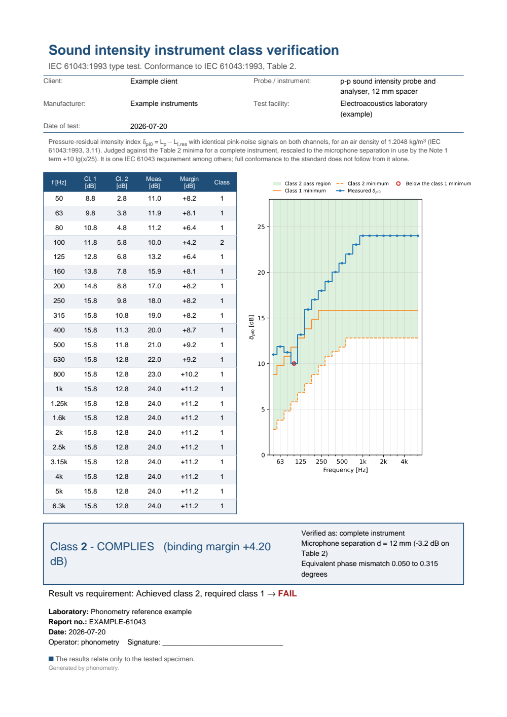
One-page instrument-class-verification fiche: a metadata header, a per-band table listing the class 1 and class 2 minima, the measured residual index, the margin and the class achieved in each one-third-octave band from 50 Hz to 6.3 kHz, the measured index drawn as a step curve over the two Table 2 masks with the 100 Hz band ringed below the class 1 minimum, the boxed Class 2 - COMPLIES (binding margin +4.20 dB) result, the microphone separation and equivalent phase mismatch, and a FAIL verdict against the required class 1.
Reading δpI0 as a phase error
Section titled “Reading δpI0 as a phase error”The requirement is really a phase-matching requirement in disguise. In an axially propagating plane wave the true phase difference across the spacer is , so a residual intensity produced by a channel mismatch gives
and the two conversions run both ways:
from phonometry import emission
# 20 dB of residual index at 1 kHz over a 25 mm spacer:phi = emission.phase_mismatch_from_residual_index(20.0, 1000.0, 0.025)print(round(float(phi), 2))     # 0.26 degrees, a hundredth of kd
# And back, for a chain whose channels are matched to 0.05°:print(round(float(emission.residual_index_from_phase_mismatch(    0.05, 1000.0, 0.012)), 1))  # 24.0 dB
That is why the low-frequency end of Table 2 rises 1 dB per third-octave band and then flattens: below the knee the standard is asking for a constant phase match, and above it for a constant index. The knee sits at 250 Hz for the three class 1 columns and for the class 2 processor, and at 630 Hz for the class 2 probe and the class 2 complete instrument, which is also where the table stops stepping in whole decibels (the instrument goes 14 dB at 315 Hz, 14.5 dB at 400 Hz, 15 dB at 500 Hz). It is also why a tenth of a degree of channel mismatch is a demanding specification, and why a probe must be verified with the spacer it will actually be used with.
Sound power at discrete points (ISO 9614-1)
Section titled “Sound power at discrete points (ISO 9614-1)”Everything above qualifies a measurement. ISO 9614-1 is the part that turns it into a sound power level, and it is the ordinary way of using a p-p probe: hold it still at each of points, one per segment of a surface enclosing the source, and read the signed normal intensity there. The partial power of a segment and the sound power of the source are then (Formulae (11) and (12)):
Formula (12) prints without the absolute-value bars that the general definition (Formula (8)) carries, because clause 9.2 disposes of the negative case instead: the method is not applicable to a band in which the sum is negative. One segment carrying inward flow is a different matter, and is normal; it is what measures.
A.2.3 makes a second refusal, and on a different quantity: where
is negative, “the test conditions do not satisfy the
requirements of this part of ISO 9614 in that frequency band”. That sum is
unweighted over the positions, while clause 9.2 weights each segment by
its area, so equal segments make the two refusals agree and unequal ones let
them part company: a band clause 9.2 keeps, with a positive total power and a
finite level, can still be one A.2.3 refuses. Its Annex A indicators come back
NaN and the determination warns, because nothing else in the result flags
it.
Both refusals are on a sum that is not positive, which is wider than the word the clauses use. A sum of exactly zero is not negative and is refused all the same: clause 9.2’s level would be , and A.2.3’s mean is the denominator of equations (A.7) to (A.9), so neither has anything to report there.
Clause 8.2 sizes the position set: at least one position per square metre and at least ten in all, distributed as evenly as the segment areas allow. Both relaxations the clause offers (one position per 2 m² where extraneous noise is significant, fifty positions over a surface larger than 50 m²) end at fifty positions, so a sparser set than that is worth saying so about, and the determination warns.
import numpy as npfrom phonometry import emission
# Measurement surface: a 2.0 m x 1.8 m x 1.4 m box over a reflecting floor,# five faces and 14.24 m2 in all, sampled at 16 positions.segment_areas = np.array([0.9] * 4 + [0.9333] * 6 + [0.84] * 6)frequencies = np.array([125.0, 250.0, 500.0, 1000.0, 2000.0, 4000.0])
# The field: nearly uniform pressure, a reactivity that grows towards low# frequency, and two positions of the 125 Hz band through which power flows# back in.rng = np.random.default_rng(9614)reactivity = np.array([9.5, 7.0, 5.0, 4.0, 3.2, 3.0])pressure_levels = 82.0 + rng.normal(0.0, 0.6, (16, 6))band_mean = 10.0 ** ((82.0 - reactivity) / 10.0) * 1e-12normal_intensity = band_mean * (1.0 + rng.normal(0.0, 0.22, (16, 6)))normal_intensity[:2, 0] = -0.4 * band_mean[0]
power = emission.sound_power_intensity_points(    normal_intensity,    segment_areas,    pressure_levels=pressure_levels,    pressure_residual_index=19.0,    frequencies=frequencies,    band_type="octave",)print(np.round(power.sound_power_level, 1))  # [83.3 86.8 88.1 89.6 90.4 90.4]print(round(power.sound_power_level_a, 1))   # 96.1 dB(A)print(round(power.surface_area, 2), power.positions)   # 14.24 16
The sign is in the print, not in the number
Section titled “The sign is in the print, not in the number”ISO 9614-1 never prints a signed level. A normal intensity level is written
XX dB when the flow through the segment is outward and (-) XX dB when it is
inward, with XX a positive number in both cases (clause 3.5, and the two
unnumbered equations of clauses 9.1 and A.2.3):
So a caller reading a printed table has to carry the sign separately, which is
what the negative argument is for. It broadcasts, so one position of a
surface can flow inward while the rest flow outward:
inward = emission.normal_intensity_from_levels(66.0, negative=True)print(f"{inward:.3e}") # -3.981e-06 W/m2, flowing inWhich grade the determination reaches
Section titled “Which grade the determination reaches”Annex B numbers two criteria, not three. Figure B.1 gates the determination on four questions, in this order, and Table B.3 says what to change when each one fails:
| Gate | Where | Action when it fails |
|---|---|---|
| Table B.3 | (e) | |
| (criterion 1) | Formula (B.1) | (a) or (b) |
| dB | Figure B.1 | (a) or (b) |
| (criterion 2) | Formula (B.2) | (c) or (d) |
Only the first failing gate is acted on: every action box in Figure B.1
returns to the next measurement rather than to the gate below it, so
required_actions() reports one action set per band and stops there. Two
codes mean the standard offers a choice, which is how Table B.3 prints them
(“a or b”).
print(power.dynamic_capability_index[0]) # 9.0 dB (Ld = 19 - 10)print(np.round(power.f2, 1)) # [9.6 6.8 5.3 3.9 3.1 3.3]print(power.criterion_1) # [False True True True True True]print(list(power.achieved_grade))# ['none', 'precision', 'precision', 'precision', 'precision', 'precision']codes = ["".join(a.value for a in band) for band in power.required_actions()]print(codes) # ['ab', '', '', '', '', '']print(power.required_actions()[0][0].criterion) # F2 > Ld or (F3 - F2) > 3 dBThe 125 Hz band is the interesting one. Its of 9.6 dB sits just above the
instrument’s dynamic capability of 9 dB, so criterion 1 fails there and no
amount of averaging will fix it: Table B.3 offers moving the surface (a) or
shielding it (b). Clause 10.5 b) then omits that band from the A-weighted
determination and asks for the omission to be stated, which
a_weighting_omitted_bands is:
print(power.a_weighting_omitted_bands) # [ True False False False False False]Grade 3 is an A-weighted determination
Section titled “Grade 3 is an A-weighted determination”Table B.2 tabulates the criterion-2 factor band by band for grades 1 and 2 and gives grade 3 one A-weighted value, 8, and no band column at all. Table B.1 does the same with the error factor (0.20 and 0.29 for all bands, 0.60 A-weighted) and Table 2 with the standard deviation of the determination. Three tables agree, so this is the standard’s design rather than a gap in it: a per-band determination reaches grade 1 or grade 2, and grade 3 is reached, if at all, by the A-weighted sum. Asking for a per-band grade-3 figure raises rather than returning a plausible number.
print(emission.position_count_factor("engineering", 1000.0, band_type="octave")) # 29.0print(emission.position_count_factor("survey")) # 8.0 (A-weighted)print(power.achieved_grade_a, round(power.field_nonuniformity_a, 2))# precision 0.13The A-weighted determination has a field non-uniformity of its own: B.1.2 sums
the A-weighted band intensities of each position into one intensity per
position and applies Formulae (A.8) and (A.9) to those, which is
field_nonuniformity_a.
The uncertainty of the result is Table 2’s , with footnote 1 placing the
true level within of the measured one at 95 % confidence. Clause 10.6
says which row of the table to read it in: the grade achieved in the final
test, not the grade the determination set out for, so expanded_uncertainty
follows achieved_grade band by band. Five bands here reached grade 1 and
carry its figures; 125 Hz reached no grade, Table 2 prints no for that, and
what clause 10.5 c) offers such a band instead is the 95 % confidence interval
of Formula (B.3), which is also what accompanies a band recorded after failing
criterion 2:
print(power.expanded_uncertainty) # [nan 3. 3. 2. 2. 2.] dBprint(np.round(power.confidence_interval[0], 1)) # [-1.7 1.2] dB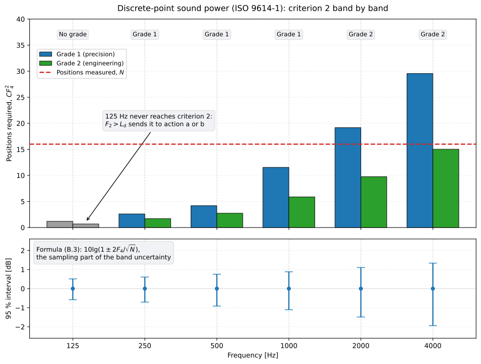
The grade is a position budget, and it is spent band by band. The survey drawn here is a second one, of a machine that radiates unevenly, and one quantity sets both of its panels: the field non-uniformity decides how many positions criterion 2 asks for, and how wide Formula (B.3) opens the interval. Its field grows less uniform with frequency, as a source whose radiation turns directional will, so the top two bands ask more than the sixteen positions measured at grade 1 and settle for grade 2, while 125 Hz never reaches criterion 2 at all: its is already above the instrument’s , and Figure B.1 sends it to an action box instead. Grade 3 is on neither panel, because Table B.2 gives it no per-band to draw.
Show the code for this figure
import matplotlib.pyplot as pltimport numpy as npfrom phonometry import emission
# The figure's own survey, which is not the example above: sixteen positions# over a 1.2 m x 0.8 m x 1.0 m machine on a reflecting floor, measured at the# 0.5 m the standard asks for, so the box is 2.2 m x 1.8 m x 1.5 m and# 15.96 m2. The field is written from its two indicators rather than drawn at# random. F2 widens towards low frequency as the field turns reactive; F4# widens towards high frequency as the radiation grows directional and the# flow concentrates on part of the surface, which is the growth criterion 2 is# about.freqs = np.array([125.0, 250.0, 500.0, 1000.0, 2000.0, 4000.0])areas = np.concatenate([np.full(4, 3.96 / 4),    # top, 2.2 m x 1.8 m                        np.full(6, 3.3 / 3),     # the two long sides                        np.full(6, 2.7 / 3)])    # the two endssurface_pressure = 84.0nonuniformity = np.array([0.25, 0.30, 0.38, 0.45, 0.58, 0.72])   # target F4pressure_intensity = np.array([11.5, 8.0, 6.0, 4.5, 3.5, 3.0])   # target F2rng = np.random.default_rng(9614)spread = rng.normal(0.0, 1.0, (areas.size, freqs.size))spread = (spread - spread.mean(axis=0)) / spread.std(axis=0, ddof=1)mean_intensity = 10.0 ** ((surface_pressure - pressure_intensity) / 10.0) * 1e-12normal_intensity = mean_intensity * (1.0 + nonuniformity * spread)
survey = emission.sound_power_intensity_points(    normal_intensity, areas,    pressure_levels=np.full((areas.size, freqs.size), surface_pressure),    pressure_residual_index=20.0,    # Ld = 20 - 10 = 10 dB (Table 1, octaves)    frequencies=freqs, band_type="octave",)
# One line — the band sound power spectrum, with the bands outside the method# hatched and the A-weighted total in the title:survey.plot()plt.show()
# The qualification figure above, by hand, from the fields the result carries# and the Table B.2 factor the module exposes.bands = np.arange(freqs.size)required = {    grade: np.array([emission.position_count_factor(grade, float(f),                                                    band_type="octave")                     for f in freqs]) * survey.f4 ** 2    for grade in ("precision", "engineering")}fig, (axt, axb) = plt.subplots(2, 1, sharex=True)for offset, grade, color in ((-0.18, "precision", "#1f77b4"),                             (+0.18, "engineering", "#2ca02c")):    axt.bar(bands + offset, required[grade], width=0.36, color=color)axt.axhline(survey.positions, color="#d62728", linestyle="--")axt.set_ylabel("Positions required, $C F_4^2$")interval = survey.confidence_intervalaxb.errorbar(bands, np.zeros_like(bands, dtype=float),             yerr=np.vstack([-interval[:, 0], interval[:, 1]]), fmt="o", capsize=6)axb.set_ylabel("95 % interval [dB]")axb.set_xticks(bands)axb.set_xticklabels([f"{f:g}" for f in freqs])axb.set_xlabel("Frequency [Hz]")plt.show()
Spending fewer new positions when the power is concentrated
Section titled “Spending fewer new positions when the power is concentrated”Where criterion 1 holds, criterion 2 does not and dB, little power is flowing inward, so most of it may be leaving through a minority of the segments. Clause 8.3.2 and B.1.3 make that testable: rank the positive partial powers, take the top segments until more than half the total power is accounted for, and require that subset to be fewer than half the segments. Then evaluate the field non-uniformity separately over the subset and over the remainder and size the new positions with Formula (B.4):
is the share of the Table B.1 error budget left for the subset
once the remainder, measured at its existing density, has taken its own, so a
remainder too non-uniform to leave anything over exhausts the budget and the
procedure cannot help. That case is refused, and so are three others: no
subset satisfying B.1.3’s two conditions, a subset of a single segment (over
one position Formula (A.8) has no spread, so Formula (B.4) has no
to square), and a remainder whose own algebraic mean is not positive. Each
refusal says which of the four it is. None of them names a row of Table B.3:
where the subset cannot be found, B.1.3 asks for “alternative appropriate
actions to increase the accuracy of sound power determination according to
table B.3”, and where the selective modification cannot be implemented, clause
8.3.2 asks for “alternative appropriate action according to B.2 and table
B.3”. Which row applies also turns on criterion 2 and on , and
partial_power_concentration is given neither.
# One band, twelve segments, most of the power through the first four.concentrated = np.array([3.0e-5, 2.4e-5, 1.8e-5, 1.4e-5] + [8.0e-6] * 8)subset = emission.partial_power_concentration(concentrated, np.full(12, 1.0))print(subset.subset_positions, round(subset.power_fraction, 2)) # 4 0.57print(subset.additional_positions) # 2Choosing the probe
Section titled “Choosing the probe”Two decisions are made before any data is taken: where the measurement surface can be placed, and which spacer goes on the probe.
Reactive fields near sources
Section titled “Reactive fields near sources”Close to a source the field turns reactive: pressure and particle velocity drift toward quadrature, so a large pressure carries little net flow. For a small source the quadrature component grows as ; at 100 Hz and 0.25 m from the source it is already about twice the active one, and climbs just as it does in the standing wave of the two-panel figure at the top of this page. The same happens between a machine and a hard reflecting surface, and in reverberant rooms where the diffuse field raises pressure without transporting energy outward. This is why ISO 9614-1 keeps the measurement surface on average more than 0.5 m away from the source, and why, when a scan fails the dynamic-capability criterion, moving the surface outward or adding absorption to the room usually lowers below more cheaply than better hardware.
Choosing the spacer
Section titled “Choosing the spacer”The spacer sets both ends of the usable band, in opposite directions:
- The top end is geometry. The finite difference underestimates the
gradient by , so the ceiling scales as
:
max_valid_frequencykeeps the bias within about 0.3 dB, giving roughly 5.7 kHz for a 6 mm spacer, 2.9 kHz for 12 mm and 690 Hz for 50 mm (bias_correct=Trueundoes the known bias somewhat beyond that). - The bottom end is phase. A progressive wave puts only degrees of true phase across the spacer, 0.8° at 63 Hz over 12 mm, while the channel mismatch stays fixed. Lowering the frequency shrinks the signal, not the error, so the margin over collapses at low frequency. A larger spacer buys back that margin: the IEC 61043 residual-index requirements scale as , so doubling the spacer is worth 3 dB of low-frequency margin.
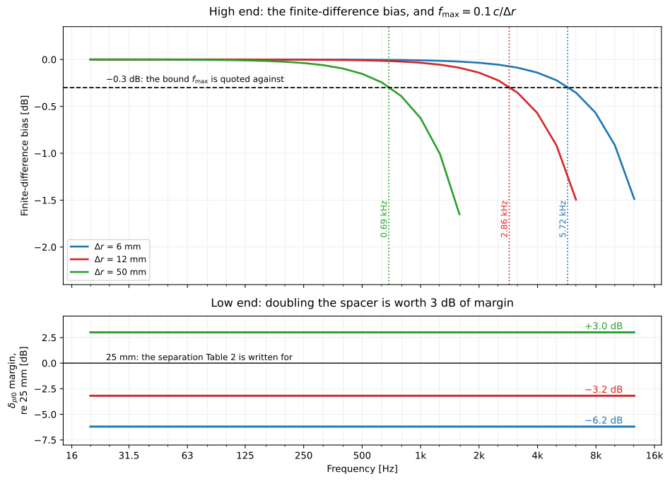
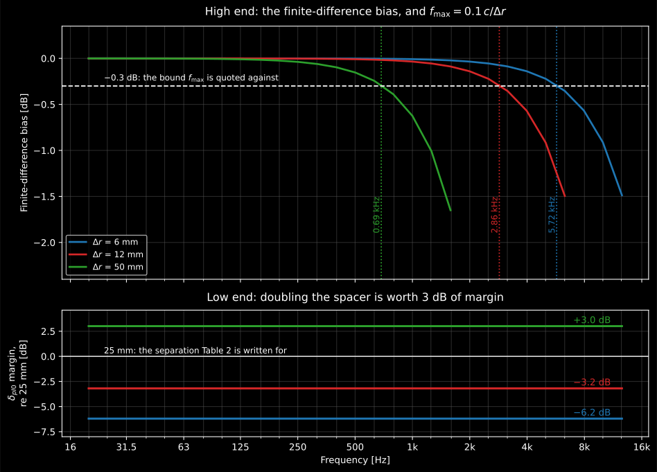
The two limits close in from opposite sides. The upper panel is geometry: each
spacer’s max_valid_frequency is exactly where its own bias curve crosses
−0.3 dB. The lower panel is the phase budget: the requirement moves with the
spacer by , so a 50 mm probe starts 3 dB
better off than a 25 mm one and 9 dB better off than a 6 mm one. Where the two
panels leave a spacer usable is the band it may be trusted over.
Show the code for this figure
import matplotlib.pyplot as pltimport numpy as np
# The bias comes out of sound_intensity itself: bias_correction is the# compensating factor (k dr)/sin(k dr), so the bias is its reciprocal in dB.fs, c = 48000, 343.0rng = np.random.default_rng(61043)x = rng.standard_normal(fs)spectrum, bins = np.fft.rfft(x), np.fft.rfftfreq(fs, 1 / fs)
fig, (axt, axb) = plt.subplots(2, 1, sharex=True)for dr in (0.006, 0.012, 0.050):    p2 = np.fft.irfft(spectrum * np.exp(-2j * np.pi * bins * dr / c), fs)    res = emission.sound_intensity(x, p2, fs, spacing=dr, fraction=3,                                   limits=[20.0, 12500.0])    usable = res.frequencies < c / (4.0 * dr)      # drop the clamped bands    axt.semilogx(res.frequencies[usable],                 -10.0 * np.log10(res.bias_correction[usable]),                 label=f"{dr * 1000:.0f} mm")    axt.axvline(res.max_valid_frequency, linestyle=":")    axb.semilogx(res.frequencies,                 np.full(res.frequencies.shape, 10.0 * np.log10(dr / 0.025)))axt.axhline(-0.3, linestyle="--")axt.set(ylabel="Bias [dB]", ylim=(-2.4, 0.35))axb.set(xlabel="Frequency [Hz]", ylabel="δpI0 margin re 25 mm [dB]")axt.legend()plt.show()
No single spacer covers the full audio range: 6 mm suits high-frequency work, 50 mm low-frequency work, and the common 12 mm covers the mid band. Wide-band surveys are measured twice with two spacers and the band results merged; whichever spacer is fitted, verify with that spacer in place, since the index belongs to the probe-spacer-analyzer chain, not to the microphones alone.
sound_intensity() parameters
Section titled “sound_intensity() parameters”| Parameter | Type | Units | Range / default | Notes |
|---|---|---|---|---|
p1, p2 | 1D arrays | Pa | equal length | Microphone closer to the source first; reversing them flips the sign |
fs | int | Hz | > 0 | |
spacing | float | m | > 0 | Microphone separation (typ. 6/12/50 mm) |
density | float | kg/m³ | default 1.204 | Air density |
speed_of_sound | float | m/s | default 343.0 | Speed of sound (bias/validity estimates) |
fraction | int, optional | — | 1, 3 or None (default) | Octave/third-octave band integration |
limits | list, optional | Hz | default library band range | Band analysis limits |
bias_correct | bool | — | default False | Apply the per-bin correction (IEC 61043 §7.3) before summing, so band/broadband totals stop under-reading as max_valid_frequency; bins past the first null are left uncorrected. The per-band bias_correction factor is reported either way |
See Theory for the derivations and Calibration for absolute scaling of the two channels.
What this guide covers
Section titled “What this guide covers”Covered
IEC 61043:1993 (EN 61043:1994) for the two-microphone cross-spectral intensity estimator of
sound_intensity, the finite-difference bias correction and its usable-bandwidth bound (clause 7.3, Table 3), the residual pressure-intensity index as the instrument’s phase-error floor, and the instrument grading built on it: the Table 2 minima per band for probes, processors and instruments with the Note 1 separation rule, the clause 6.1 frequency ranges and the clause 8 component-combination rule (verify_intensity_class,residual_index_limits,instrument_class_from_components), plus the to phase-mismatch conversion in both directions. ISO 9614-1:1993 for the Annex A field indicators to (temporal_variability_indicator,field_indicators) with the Table B.3 limit on , and the Annex B dynamic-capability criterion (dynamic_capability_index); and its own discrete-point sound-power determination, clauses 8 and 9, which sums the partial powers into (Formulae (11) and (12)) and qualifies it against Annex B: criterion 1, the inward-flow gate of Figure B.1 and criterion 2 with the Table B.2 factor , the Table B.3 actions, the Formula (B.3) confidence interval, the Table 2 uncertainty and the optional concentration procedure of clause 8.3.2 (sound_power_intensity_points,position_count_factor,determination_standard_deviation,error_factor,normal_intensity_from_levels,partial_power_concentration).Not covered
The residual-intensity test of IEC 61043 is not performed by the library: is a value the caller measures on their own probe-analyzer chain, with the spacer that will be fitted, and supplies: the procedure is in Measuring the residual index above, and what phonometry does with the number is grade it against Table 2. The before-use check of clause 14 and the ISO 9614-2 probe-reversal test are likewise procedures, not functions.
References
Section titled “References”- Fahy, F. J. (1995). Sound intensity (2nd ed.). E&FN Spon. https://doi.org/10.4324/9780203475386ISBN 978-0-419-19810-9. The monograph on the subject: active and reactive intensity, the p-p estimator and the phase-mismatch error budget behind this page.
- International Electrotechnical Commission. (1993). Electroacoustics — Instruments for the measurement of sound intensity — Measurements with pairs of pressure sensing microphones (IEC 61043:1993). Adopted in Europe as EN 61043:1994. The instrument standard: the two-microphone cross-spectral estimator, the residual-intensity test behind δpI0, the Table 2 minimum residual index per band for probes, processors and instruments in class 1 and class 2 with its +10 lg(x/25) separation rule (Note 1), the processor frequency ranges (clause 6.1), the component-combination rule (clause 8), and the finite-difference bias correction with its usable-bandwidth bound (clause 7.3, Table 3).
- International Organization for Standardization. (1993). Acoustics — Determination of sound power levels of noise sources using sound intensity — Part 1: Measurement at discrete points (ISO 9614-1:1993). The pressure-intensity index, the Annex A field indicators F1 to F4 (F1 from equations (A.1)-(A.2), evaluated in the initial test of clause 8.2 and again per B.1.4), the Table B.3 temporal-variability limit, the dynamic-capability criterion (Annex B) and the 0.5 m surface-distance rule.