Sound power from surface vibration (ISO/TS 7849)

Standards: ISO/TS 7849Key references: Cremer et al. 2005

The airborne sound power a machine radiates through the structure-borne vibration of its outer surface can be estimated from the surface vibratory velocity and a radiation factor $ε$ (the radiation efficiency), without an acoustic measurement. The radiated power is (ISO/TS 7849-1, Formula 6)

P = Z_{c} ⟨ v^{2} ⟩ S ε [W],

with $Z_{c}$ the characteristic impedance of air, $⟨ v^{2} ⟩$ the mean-square vibratory velocity over the radiating area $S$ . Expressed in levels (velocity level re $v_{0} = 5 \times 1 0^{- 8} m/s$ ), each part writes that relation in its own quantities. Part 1 is A-weighted throughout: one A-weighted surface velocity level $L_{v A}$ , the fixed $ε_{A} = 1$ , and a single A-weighted number, the upper limit of the airborne sound power level (Formula 12)

L_{W A, m a x} = L_{v A} + 10 lo g_{10} \frac{S}{S _{0}} + 10 lo g_{10} \frac{Z _{c, n}}{Z _{c, 0}} .

Part 2 is the band-wise counterpart, with the radiation factor $ε_{j}$ determined for each band (Formula 15)

L_{W, j} = L_{v, j} + 10 lo g_{10} \frac{S}{S _{0}} + 10 lo g_{10} ε_{j} + 10 lo g_{10} \frac{Z _{c, n}}{Z _{c, 0}},

where $S_{0} = 1 m^{2}$ , the normalized impedance $Z_{c, n} = 411 N\cdots/m^{3}$ and the reference $Z_{c, 0} = 400 N\cdots/m^{3}$ give the fixed $10 lo g_{10} (411/400) = 0.118 dB$ term. This guide runs the band-wise form for both parts, so that the Part 1 upper limit and the Part 2 engineering value can be compared band by band; a strict Part 1 survey is the single A-weighted number above, which the result object carries as sound_power_level_a. This module feeds the structure-borne source and building prediction standards (ISO 9611, EN 15657, EN 12354-5).

Before any levels, the radiator itself. The radiation_efficiency plate model that supplies a predicted radiation factor retains its geometry, and sigma.plot_geometry() draws the plate in its baffle to scale, here 1.5 m by 1.25 m and simply supported.

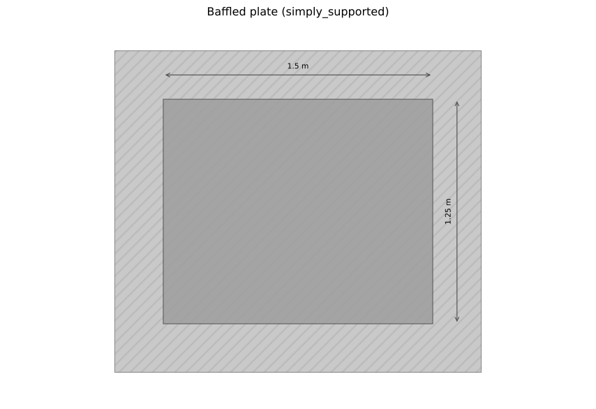
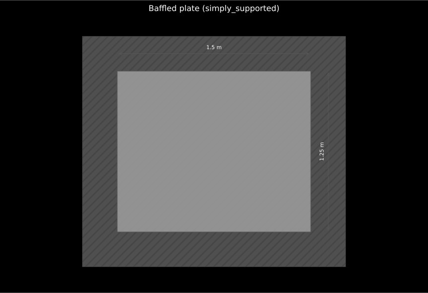
To-scale front view of the plate of the radiation model: a grey 1.5 m by 1.25 m simply supported plate inside its hatched rigid baffle, both side lengths dimensioned and the boundary condition named in the title

The radiator behind the radiation factor, to scale: the 1.5 m by 1.25 m simply supported plate in its rigid baffle, whose area $S$ enters $L_{W}$ directly while its size decides how far $ε$ falls below one under coincidence.

Show the code for this figure

import matplotlib.pyplot as plt
import numpy as np
from phonometry import vibration

# The simply supported 1.5 x 1.25 m plate of the radiation model.
f = np.geomspace(50.0, 5000.0, 200)
sigma = vibration.radiation_efficiency(f, 1.5, 1.25, 2100.0)
sigma.plot_geometry()
plt.show()

1. The two parts

The two parts differ only in the radiation factor. Part 1 (survey) assumes $ε = 1$ and yields the upper limit $L_{W, m a x}$ , needing only the velocity level and the area. Part 2 (engineering) applies a frequency-band radiation factor $ε_{j}$ determined (per ISO 9614) as $ε_{j} = P_{j} / (Z_{c, n} ⟨ v_{j}^{2} ⟩ S)$ .

import numpy as np
from phonometry import emission

bands = np.array([250.0, 500.0, 1000.0, 2000.0])
lv = np.array([82.0, 85.0, 83.0, 79.0])          # mean velocity level per band [dB]

# Part 1 upper limit (epsilon = 1):
upper = emission.sound_power_from_vibration(lv, area=1.6, frequencies=bands)
print(round(upper.total_level, 1))               # 90.9  dB re 1 pW, unweighted
print(round(upper.sound_power_level_a, 1))       # 88.9  dB(A) re 1 pW

# Part 2 engineering value with a measured radiation factor:
eps = np.array([0.45, 0.75, 0.95, 1.00])
eng = emission.sound_power_from_vibration(lv, area=1.6, radiation_factor=eps, frequencies=bands)
print(np.round(eng.sound_power_level, 1))        # per-band L_W
print(round(eng.sound_power_level_a, 1))         # 88.4  dB(A) re 1 pW

eng.plot()   # the LW(f) spectrum, as in the figure above (needs matplotlib)

The two totals are not interchangeable: total_level is the unweighted band sum $10 l g \sum_{j} 1 0^{0.1 L_{W, j}}$ , while sound_power_level_a is the A-weighted total that the fiche boxes and that a noise declaration quotes. They differ by the A-weighting of the spectrum — 2.0 dB on this casing, several decibels more on a low-frequency-heavy one.

Set the two parts side by side on one casing and the price of Part 1’s assumption is a picture rather than an argument:

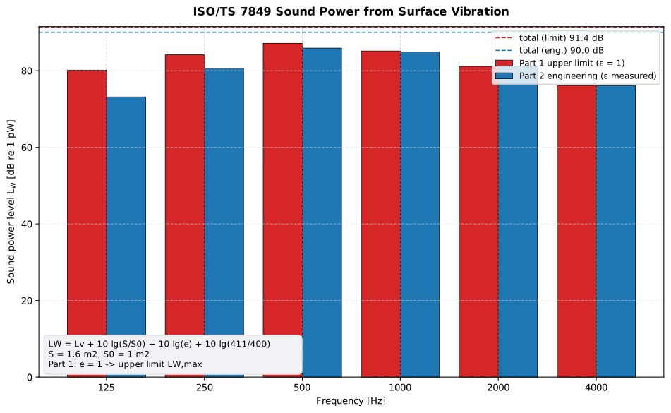
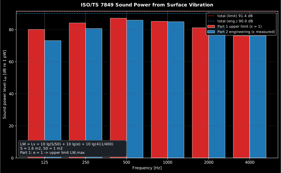
Radiated sound power level per octave band, comparing the ISO/TS 7849-1 upper limit (radiation factor of one) with the ISO/TS 7849-2 engineering value (measured radiation factor)

Paired bars per band for a 1.6 m² casing: Part 1’s upper limit against Part 2’s engineering value. The gap is $- 10 lo g_{10} ε_{j}$ — 7.0 dB at 125 Hz, 3.5 dB at 250 Hz, 1.2 dB at 500 Hz and nothing from 2 kHz up — so the error Part 1 makes is largest in the low bands, exactly where a large thin casing radiates worst.

Show the code for this figure

import matplotlib.pyplot as plt
import numpy as np
from phonometry import emission

# Surface velocity levels and a measured radiation factor per octave band.
bands = np.array([125.0, 250.0, 500.0, 1000.0, 2000.0, 4000.0])
lv = np.array([78.0, 82.0, 85.0, 83.0, 79.0, 74.0])
eps = np.array([0.20, 0.45, 0.75, 0.95, 1.00, 1.00])

lw_max = emission.radiated_sound_power_level(lv, 1.6)  # Part 1, eps = 1
lw_eng = emission.radiated_sound_power_level(lv, 1.6, radiation_factor=eps)  # Part 2

# The figure above: the two parts band by band.
x = np.arange(bands.size)
fig, ax = plt.subplots()
ax.bar(x - 0.2, lw_max, width=0.4, label="Part 1 upper limit ($\\varepsilon$ = 1)")
ax.bar(x + 0.2, lw_eng, width=0.4, label="Part 2 engineering ($\\varepsilon$ measured)")
ax.set_xticks(x, [f"{b:g}" for b in bands])
ax.set(xlabel="Frequency [Hz]", ylabel="Sound power level $L_W$ [dB re 1 pW]")
ax.legend()
plt.show()

# A single determination is a result object that draws its own spectrum:
res = emission.sound_power_from_vibration(lv, area=1.6, radiation_factor=eps,
                                          frequencies=bands)
res.plot()
plt.show()

2. Velocity level, calibration and the radiation factor

The velocity level is $L_{v} = 20 lo g_{10} (v / v_{0})$ (Formula 3); a sinusoidal calibration acceleration converts as $L_{v} = 20 lo g_{10} (\overset{a}{^} / (2 π f v_{0} 2))$ (Formula 8). The radiation factor comes from an independently measured power:

from phonometry import emission

# The standard's worked calibration EXAMPLE: 9.81 m/s^2 at 100 Hz.
print(round(float(emission.velocity_level_from_acceleration(9.81, 100.0)), 1))   # 106.9 dB

# Radiation factor from a measured power (ISO 9614): eps = P / (Zc <v^2> S).
eps = emission.radiation_factor(3.0e-4, area=2.0, mean_square_velocity=(1e-3)**2)
print(round(float(eps), 3))                                                # 0.365

Surface velocity levels from several positions are combined with the energetic mean mean_velocity_level (Formula 10) or its area-weighted form (Formula 11), and the correction extraneous_velocity_correction removes extraneous vibration per Table 2.

Those positions are not free: the standard divides the radiating surface $S$ into $N$ equal cells and puts one accelerometer at the centre of each. Table 1 fixes the initial $N$ from the area alone — 5 positions below 1 m², 10 from 1 m² to 10 m², and $S / S_{0}$ positions above that ( $S_{0} = 1$ m²) — so the 4 m² surface drawn below takes ten. Increase $N$ when the spread of the A-weighted velocity level over the positions, highest minus lowest in decibels, exceeds twice the Table 1 count; a strongly non-uniform field can instead be handled by redistributing the positions, which makes the partial areas $S_{i}$ unequal and so calls for the area-weighted Formula 11 rather than the plain energetic mean. The Table 2 correction is a ladder on the same kind of spread: with the machine stopped and the surrounding plant running, the mean extraneous velocity level must sit at least 3 dB below the machine’s, and extraneous_velocity_correction returns 3 dB at a 3 dB difference, 2 dB at 4-5 dB, 1 dB at 6-9 dB and 0 dB from 10 dB up.

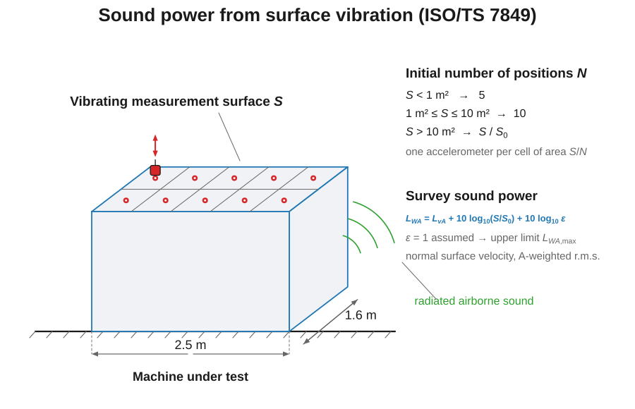
ISO/TS 7849 surface-velocity method: a machine under test with its vibrating measurement surface of 2.5 by 1.6 metres divided into ten equal cells, an accelerometer at each cell centre, the radiated airborne sound leaving the surface, the Table 1 initial number of measurement positions (5 below 1 square metre, 10 from 1 to 10, S over S0 above) and the survey relation LWA = LvA + 10 lg(S/S0) + 10 lg epsilon

The Table 2 ladder is one call on a measured difference:

# With the machine stopped and the surrounding plant running, the mean
# extraneous velocity level is 5.4 dB below the operating one.
k1a = emission.extraneous_velocity_correction(5.4)
print(k1a)                                        # 2.0 dB, subtracted from Lv
print(round(float(np.mean(lv)) - k1a, 1))         # 80.2 dB after the correction

Mounting the transducer

Everything above assumes $L_{v}$ is the surface’s own normal velocity. Whether it is depends on the transducer and on how it is attached, and both have a frequency limit that is easy to exceed without any warning in the data.

Use a piezoelectric accelerometer light enough not to mass-load the panel, and only over the flat part of its response: the usable upper limit is about one third of the transducer’s own mounted resonance, which keeps the reading within roughly 1 dB. A 30 kHz-resonance miniature accelerometer is therefore good to about 10 kHz; a heavy 6 kHz one only to 2 kHz. Mount it per ISO 5348 with its sensitive axis normal to the surface, because the method needs the normal component and nothing else, and fix the cable to the machine close to the transducer so that cable motion does not drive the charge amplifier.

The attachment is the part that silently costs bandwidth:

Attachment	Usable to	Notes
Stud (threaded)	the transducer’s own limit	The reference mounting; needs a drilled and faced boss
Adhesive, or a thin layer of adhesive wax	about 10 kHz	Wax not on hot surfaces (it softens well below 40 °C)
Clamping magnet	about 2.5 kHz	Smooth flat steel only; a 110 g magnet plus a 30 g transducer also caps the measurable acceleration, and paint or roughness destroys the adhering force
Hand-held probe	low bands only	For a quick survey, never for a determination

That table has a direct consequence for the examples on this page, which run octave bands out to 4 kHz: a magnet mount loses the top band outright, and loses it quietly — the level simply reads low rather than failing a check. A scanning laser vibrometer avoids the mass loading and the mounting limit altogether, provided the beam stays perpendicular to the surface, since it too measures only the component along the beam.

3. When the radiation-factor assumption breaks

The whole method stands on one substitution: replacing the acoustic measurement by $ε$ . The Part 1 value $ε = 1$ is close to the true radiation factor only above the critical (coincidence) frequency of plate-like parts, where bending waves travel faster than sound and the surface radiates like a piston. Below coincidence, adjacent zones of the plate move in antiphase and their radiation largely cancels: $ε$ drops far below one and falls quickly with decreasing frequency, so the survey method can overstate the low-frequency bands of a large thin casing by 10 dB and more. The same cancellation makes small sources radiate poorly (the acoustic short circuit around an unbaffled panel). Two further assumptions are easy to violate in the field:

The measured vibration must be the machine’s own. Vibration fed in from neighbouring machinery inflates $⟨ v^{2} ⟩$ ; Table 2 prescribes the source-off check and extraneous_velocity_correction applies it.
The surface must be the dominant radiator. Airborne sound from openings, intakes or internal sources that bypasses the measured casing is invisible to a velocity survey; the method characterises the structure-borne part only.

What the cancellation looks like

“Adjacent zones move in antiphase and their radiation largely cancels” is the sentence the whole caveat rests on, and it is a statement about a phase relationship between a travelling structural wave and the air on top of it — which a spectrum cannot draw. The clip below drives a 10 mm steel plate in air along its whole length, with a force on the plate rather than a wave arriving at it, because that is the emission case this method is about — and because a plate driven only over a patch radiates from the patch, which below coincidence would be the only thing in the air and would teach the opposite of the truth. It then runs the same scene twice, at $f_{c} /2$ and at $2 f_{c}$ , with nothing differing between the panels but the drive frequency.

Download the animation (WebM)

Below coincidence the bending wavelength is shorter than the acoustic one. Adjacent half-waves of the plate push and pull the same air in antiphase, and what the air shows is a skin of alternating lobes that clings to the plate and dies within a fraction of a wavelength. The pressure at the surface is of the same order as in the other panel; it is simply a quarter-cycle out of step with the velocity, so it carries no power away — which is what $ε ≪ 1$ means. Above coincidence the bending wave outruns sound, the trace match is satisfied, and a plane beam leaves at $arcsin (c_{0} / c_{B}) = 45°$ .

Each panel is annotated with the closed forms its regime obeys, taken from the plate’s own constants: below coincidence, that $λ_{B} = 0.40$ m is shorter than the 0.57 m of sound in air, so $sin θ = λ / λ_{B}$ has no solution — there is no angle for the sound to leave at — and the skin that stands in its place decays with a height of $1/ k_{B}^{2} - k_{0}^{2} = 0.091$ m; above coincidence, that $λ_{B} = 0.20$ m is longer than the 0.14 m in air, so the trace match is satisfied and sends a beam out at 45°. Nothing is measured off the scene itself. Two quantities were tried and both were spoiled by the ends of the plate — a damping layer reflects a bending wave partially, so the air carries a leftward beam on top of the rightward one, and the reading is the difference of the two rather than either. Terminating a bending wave well enough to read a number off it needs a much wider domain than a picture of this can hold.

Two cautions on reading it. The scene is an effectively infinite plate in air, so what it demonstrates is below-coincidence cancellation, not the acoustic short circuit around an unbaffled panel: those are the same cancellation at two different scales, and the second one needs a finite source with a path around its edge. And the clip deliberately does not print a radiation factor. A $ε$ read off a scene like this would be an artefact of the drive: any finite driving aperture has a wavenumber spectrum broad enough to put some of itself inside the radiating region, and below coincidence that aperture radiation would be the only thing crossing an intensity line, since the travelling subsonic wave contributes exactly nothing. The number belongs to the closed-form curve in the next subsection; the clip is here for the mechanism behind it.

Estimating the radiation factor before you measure it

None of that has to be taken on trust: the library predicts $ε$ for a plate, and it is the same radiation_efficiency model that drew the plate at the top of this page. The critical frequency follows from the surface mass and the bending stiffness — a 3 mm steel panel puts it near 4 kHz — and it is where bending waves travel at the speed of sound and the plate begins to radiate like a piston. Everything below it is the acoustic short circuit.

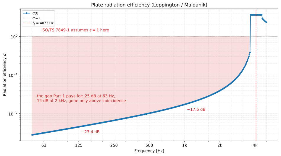
The radiation efficiency sigma of the 1.5 by 1.25 metre plate on log-log axes from 50 Hz to 5 kHz, rising from about 0.003 at 63 Hz to a peak just above the critical frequency of 4073 Hz. The whole region below the sigma equals one line is shaded and labelled as the range where ISO/TS 7849-1 assumes epsilon equals one, with the radiation index marked at minus 23.4 dB at 125 Hz and minus 17.6 dB at 1 kHz

The shaded area is the assumption Part 1 makes. For this plate it is worth 25 dB at 63 Hz and 14 dB at 2 kHz, and it closes only at coincidence — which is the “10 dB and more” of the paragraph above, drawn.

Show the code for this figure

import matplotlib.pyplot as plt

# The same 1.5 x 1.25 m plate, now as a 3 mm steel panel so the coincidence
# frequency comes from the material rather than being assumed.
f = np.geomspace(50.0, 5000.0, 400)
stiffness = vibration.plate_bending_stiffness(2.0e11, 0.003, 0.30)
fc = vibration.coincidence_frequency(7800.0 * 0.003, stiffness)
print(round(fc, 0))                                   # 4073.0 Hz
sigma = vibration.radiation_efficiency(f, 1.5, 1.25, fc)
print(round(float(np.interp(1000.0, f, sigma.radiation_index)), 1))    # -17.6 dB

sigma.plot()          # sigma(f) with the sigma = 1 line and fc marked
plt.show()

A predicted $ε$ feeds straight back into the determination: sound_power_from_vibration(lv, area=…, radiation_factor=sigma.radiation_efficiency, frequencies=bands) turns a Part 1 survey into a first estimate of the Part 2 value. Take it for what it is — a baffled flat plate with a known boundary condition is not a machine casing with ribs, apertures and a gearbox bolted to it — but it is enough to know whether the Part 1 number is 1 dB or 15 dB pessimistic before committing to an intensity measurement. The same $ε$ appears as $σ$ , the radiation efficiency, in Panel Sound Insulation: the emission standards write it $ε$ and the building-prediction standards write it $σ$ , and it is the same quantity computed by the same function.

Part 2 exists exactly for the radiation-factor problem: it replaces the fixed $ε = 1$ with a band-by-band $ε_{j}$ determined from one reference measurement of the radiated power (ISO 9614 intensity), after which the velocity survey can be repeated cheaply on nominally identical machines.

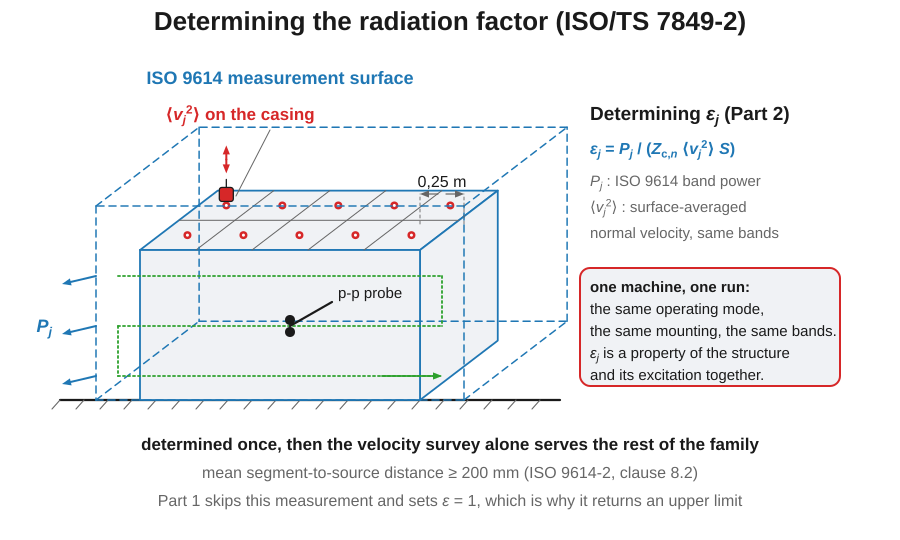
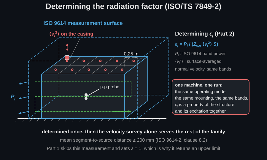
The ISO/TS 7849-2 determination of the radiation factor: the same machine casing carrying its ten-cell accelerometer grid with the mean square velocity measured on the surface, enclosed by an ISO 9614 measurement surface offset 0.25 m from it over which a p-p probe traces a serpentine sweep, the band power P_j leaving that surface, and the relation epsilon_j equals P_j divided by the characteristic impedance times the mean square velocity times the area, taken on one machine in one operating mode

That pairing is the whole of Part 2, and it is where the transferability has to be qualified. Clause 4.4.3 is explicit that $ε_{j}$ is determined not only by the geometry and the mechanical properties of the structure but also by the distribution and manner of the excitation and by the internal loss factor, so a factor measured at idle does not carry to full load, and one measured on a soft mount does not carry to a bolted installation: the operating and mounting condition is part of the $ε$ , exactly as it is part of every other emission value in this section. Clause 4.2 adds the modal caveat — in bands where only a very few modes are excited, $ε_{j}$ is set by which modes happen to be excited rather than by the surface’s average radiating behaviour, so it is unstable from run to run and from machine to machine. That makes the low bands the least transferable part of the spectrum, and they are also where the Part 1 upper limit is worst. The practical rule: reuse an $ε$ only across the same machine family, the same operating mode and the same mounting, and re-verify it on a sample.

4. The measurement report (`.report()`)

A determination ends as a document. The VibrationSoundPowerResult exposes a .report() method that writes a one-page PDF fiche laid out like a sound-power test sheet: the standard-basis line naming the applied method (the ISO/TS 7849-1 survey method with a fixed radiation factor $ε = 1$ , or the ISO/TS 7849-2 engineering method with a determined radiation factor), an optional metadata header (client, machine/source, test environment, instrumentation, climate, date), a per-band table (nominal octave/one-third-octave frequency, the surface vibratory velocity level $L_{v}$ and the band sound-power level $L_{W}$ ), the sound-power spectrum $L_{W} (f)$ with a nominal band axis, and a boxed A-weighted sound power level $L_{W A}$ (dB re 1 pW) with the total $L_{W}$ , the radiating area $S$ and the applied method alongside. Those two come from the result’s sound_power_level_a (the declarable A-weighted total) and total_level (the unweighted band sum); the table columns come from velocity_level, sound_power_level and, with verbose=True, radiation_factor.

The metadata is supplied through a ReportMetadata, whose applicable fields here are the machine/source description (specimen), the test environment (test_room), the client, the instrumentation, the temperature, relative humidity and ambient pressure, the date of test (test_date) and the footer identity (laboratory, operator, report_id, notes); the radiating area $S$ comes from the result itself and is printed in the result box, together with the sound-power relation $L_{W} = L_{v} + 10 lo g_{10} (S / S_{0}) + 10 lo g_{10} ε + 10 lo g_{10} (Z_{c, n} / Z_{c, 0})$ in the basis strip. Supplying requirement adds a PASS/FAIL verdict against a declared A-weighted sound-power limit (a sound-power emission is a quantity where less is better, so the source passes at or below the limit). verbose=True adds the radiation factor $ε$ column to the table. language="es" renders the Spanish fiche with comma decimals.

import numpy as np
from phonometry import ReportMetadata, emission

freqs = np.array([125, 250, 500, 1000, 2000, 4000], float)
lv = np.array([78.0, 82, 85, 83, 79, 74])          # surface velocity level [dB]
eps = np.array([0.20, 0.45, 0.75, 0.95, 1.00, 1.00])  # measured radiation factor
res = emission.sound_power_from_vibration(
    lv, area=1.6, radiation_factor=eps, frequencies=freqs,
)

res.report(
    "vibration_sound_power.pdf",
    metadata=ReportMetadata(
        client="Example manufacturing plant",
        specimen="Gearbox casing (steel panel)",
        test_room="Machine hall (source vibration survey)",
        instrumentation="Piezoelectric accelerometer (ISO 16063-21 calibration), s/n 0042",
        laboratory="Phonometry reference example",
        report_id="EXAMPLE-7849",
        requirement=90.0,
    ),
)   # LWA = 88.7 dB(A) re 1 pW -> declared limit 90 dB(A): PASS

The example fiche is regenerated with make reports and kept rendered in the repository; click the preview to open the PDF.

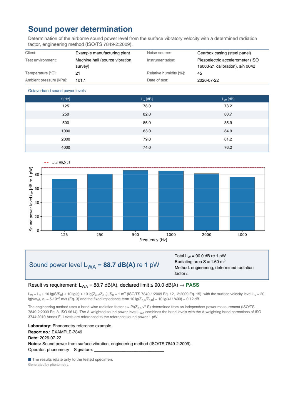
ISO/TS 7849 sound power from vibration example report (PDF) — Sound power from vibration fiche (VibrationSoundPowerResult.report), an ISO/TS 7849-2 engineering-method determination with the measured radiation factor and the boxed LWA.

What this guide covers

Covered
ISO/TS 7849-1:2009 and ISO/TS 7849-2:2009 as far as they define the calculation of sound power from vibration: the radiated power $P = Z_{c} ⟨ v^{2} ⟩ S ε$ (Formula 6), the velocity level and its calibration conversion (Formulae 3, 8) run by velocity_level and velocity_level_from_acceleration, the surface mean (Formulae 10/11) run by mean_velocity_level, the extraneous-vibration correction of Table 2 run by extraneous_velocity_correction, and the sound power level with the fixed impedance term (Formula 12, Part 1) or a measured per-band radiation factor (Formula 15, Part 2) run by radiated_sound_power_level and sound_power_from_vibration. radiation_factor implements Part 2’s single-machine Formula 8, converting an independently measured sound power into $ε$ .
Not covered
The measurement clauses of both parts (instrumentation, source installation, environmental conditions: clauses 5 to 7) are not implemented as code, and neither are their measurement-uncertainty clauses and informative annexes: they are laboratory practice, and this guide states the rules of it that decide whether the inputs are valid at all — the Table 1 position counts, the Table 2 extraneous-vibration ladder and the transducer mounting limits above. Part 2’s clause 8 also asks for the radiation factor of a machine batch or family, averaging $ε_{j}$ over several machines and its standard deviation (Formulae 9, 10); only the single-machine Formula 8 is implemented, so pass an already-averaged $ε$ for a family determination. The sound power that feeds radiation_factor must come from an ISO 9614 intensity determination, which is Sound Power by Intensity Scanning (sound_power_intensity, or sound_power_intensity_precision for grade 1) — the sound intensity guide covers the probe and the field indicators behind it but computes no power.

References

Cremer, L., Heckl, M., & Petersson, B. A. T. (2005). Structure-borne sound: Structural vibrations and sound radiation at audio frequencies (3rd ed.). Springer. https://doi.org/10.1007/b137728The radiation-efficiency treatment behind section 3: coincidence, the cancellation below the critical frequency and the radiation of finite plates. ISBN 978-3-540-22696-3.
International Organization for Standardization. (2009). Acoustics — Determination of airborne sound power levels emitted by machinery using vibration measurement — Part 1: Survey method using a fixed radiation factor (ISO/TS 7849-1:2009). The upper-limit method with ε = 1: the radiated power P = Z_c⟨v²⟩Sε (Formula 6), the velocity level and its calibration (Formulae 3, 8), the mean over the surface (Formulae 10/11), the extraneous correction (Table 2) and the sound power level with the fixed impedance term (Formula 12). Conformance is anchored on the standard's own worked calibration example.
International Organization for Standardization. (2009). Acoustics — Determination of airborne sound power levels emitted by machinery using vibration measurement — Part 2: Engineering method including determination of the adequate radiation factor (ISO/TS 7849-2:2009). The engineering method with a measured band-wise radiation factor (Formula 4/8) and its sound power level (Formula 15). Conformance includes the exact round-trip between the radiation factor and L_W = 10 lg(P/P₀).

Created and maintained by José Manuel Requena Plens ORCID All projects

Sound power from surface vibration (ISO/TS 7849)

1. The two parts

2. Velocity level, calibration and the radiation factor

Mounting the transducer

3. When the radiation-factor assumption breaks

What the cancellation looks like

Estimating the radiation factor before you measure it

4. The measurement report (.report())

What this guide covers

See also

References

4. The measurement report (`.report()`)