Quasi-peak programme meter (ITU-R BS.468-4)
Standards: ITU-R BS.468IEC 60268AES17
ITU-R BS.468-4 measures audio-frequency noise voltage in sound broadcasting with two things in series: the weighting network of clause 1, which peaks at +12.2 dB near 6.3 kHz, and the quasi-peak detector of clause 2, which is what this page is about. The result is reported in dBqps (clause 3). NOTE 1 to clause 1 is blunt about why both halves are needed: reading the weighted signal with any other meter, “e.g. an r.m.s. meter”, gives signal-to-noise figures “that are not directly comparable” with the ones the Recommendation describes.
The curve is
weighting_filter(curve="468"). The
detector is broadcast.quasi_peak_meter.
1. What clause 2 specifies, and what it does not
Section titled “1. What clause 2 specifies, and what it does not”Clause 2 gives no time constant, no rise time, no decay law and no transfer function. Its preamble says the required dynamic performance “may be realized in a variety of ways”, and the words “time constant” occur once in the whole Recommendation, inside an informative Note offering “two peak rectifier circuits of different time-constants connected in tandem” as a possible arrangement after full-wave rectification.
What clause 2 gives instead is eleven acceptance windows. Table 2 reads a single 5 kHz tone burst at eight durations from 1 ms to 200 ms; Table 3 reads a train of 5 ms bursts at 2, 10 and 100 per second. Every cell is a percentage of the reading the same tone gives steadily, so both tables are ratios and every absolute factor, the network’s +11.7 dB at 5 kHz included, cancels.
| Stimulus | Lower | Reference | Upper | Window |
|---|---|---|---|---|
| 1 ms burst | 13.5 % | 17.0 % | 21.4 % | 4.00 dB |
| 2 ms burst | 22.4 % | 26.6 % | 31.6 % | 2.99 dB |
| 5 ms burst | 34 % | 40 % | 46 % | 2.63 dB |
| 10 ms burst | 41 % | 48 % | 55 % | 2.55 dB |
| 20 ms burst | 44 % | 52 % | 60 % | 2.69 dB |
| 50 ms burst | 50 % | 59 % | 68 % | 2.67 dB |
| 100 ms burst | 58 % | 68 % | 78 % | 2.57 dB |
| 200 ms burst | 68 % | 80 % | 92 % | 2.63 dB |
| 5 ms at 2/s | 43 % | 48 % | 53 % | 1.82 dB |
| 5 ms at 10/s | 72 % | 77 % | 82 % | 1.13 dB |
| 5 ms at 100/s | 94 % | 97 % | 100 % | 0.54 dB |
Two readings of the percentage column are grammatically possible and only one survives: at 100 bursts per second the upper limit is 100 %. Under “percent of full scale”, with the steady tone reading 80 % of full scale, that limit would sit 1.94 dB above the steady tone, which no peak-following detector can reach on a 50 % duty cycle of the very same tone. Under “percent of the steady reading” it says the train “may reach but not exceed the steady reading”, which is the physical ceiling and the natural thing to print.
That last row is also the sharpest test in the document: 0.54 dB wide, against 4.00 dB at 1 ms.
2. Reading a record
Section titled “2. Reading a record”quasi_peak_meter runs the detector over a whole record and returns the
largest excursion of the reading device, which is what an operator writes down
from a pointer. The record therefore has to include the decay: a burst that
ends at the last sample is read before the needle has finished rising.
from phonometry import broadcast, signals
fs = 48000# Clause 2.2's own stimulus: 5 ms (25-period) bursts of 5 kHz at 10 per# second, at the amplitude that makes the steady tone read 0 dBqps.burst = signals.tone_burst(fs, 5000.0, 25, amplitude=0.285,                           repetitions=16, repetition_rate=10.0,                           post_silence=0.5)result = broadcast.quasi_peak_meter(burst.signal, fs)print(round(result.reading, 4))                            # 0.5872   voltsprint(round(result.level_db, 2), result.level_unit)        # -2.41 dBqps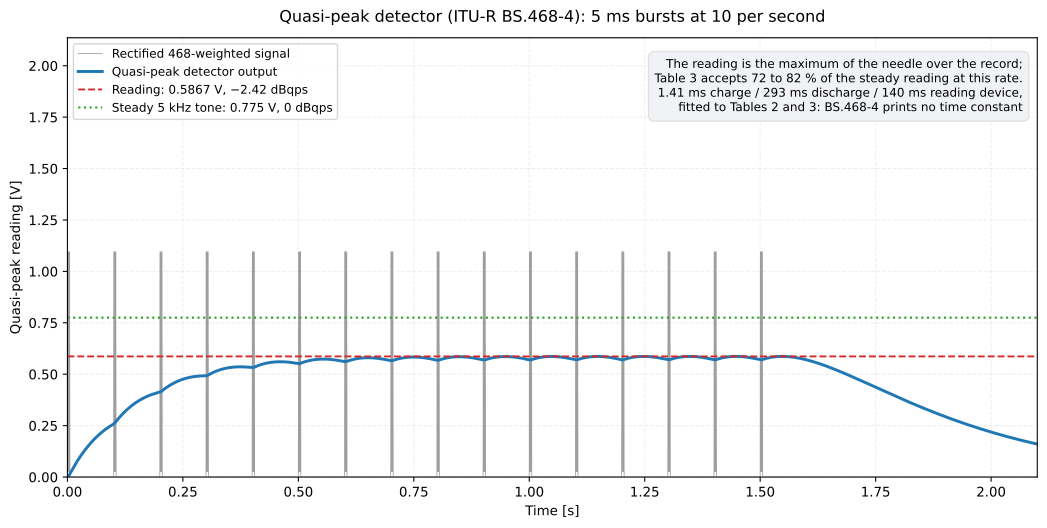
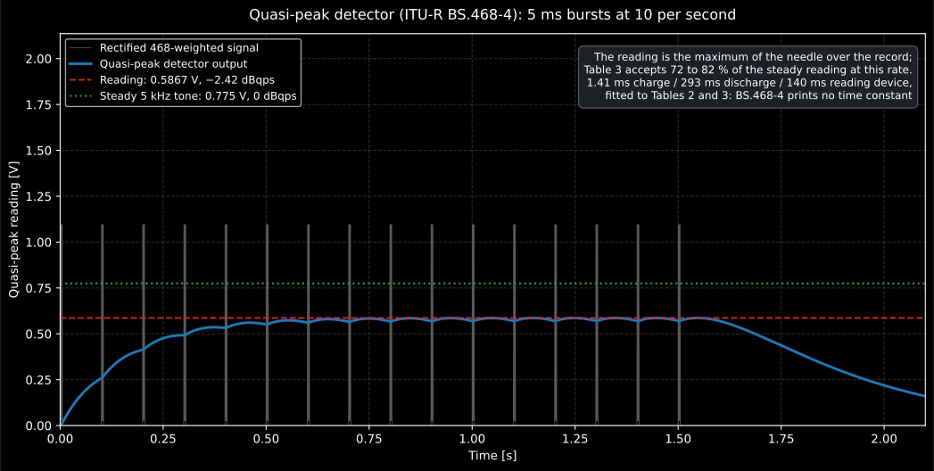
The whole content of clause 2 in one picture: the needle rises over the first half second, ripples once the charge between bursts and the decay in the gaps balance, and falls away after the train stops. The gap between the two horizontal lines is Table 3’s 10 bursts per second cell, drawn to scale: the train reads 75.8 % of the steady tone against a printed 77 %, inside the 72 to 82 % window.
Show the code for this figure
import matplotlib.pyplot as pltfrom phonometry import broadcast, signals
fs = 48000burst = signals.tone_burst(fs, 5000.0, 25, amplitude=0.285,                           repetitions=16, repetition_rate=10.0,                           post_silence=0.5)broadcast.quasi_peak_meter(burst.signal, fs).plot()plt.show()
The result carries the trace the figure draws, sample for sample with the
record, so the ballistics are visible rather than hidden behind a scalar. Set
weighted=False to take the network out of the path, which is what clause 2.4
does and the only test in clause 2 that does.
3. The scale, and when a reading is dBqps
Section titled “3. The scale, and when a reading is dBqps”Clause 2.6 is the one absolute statement in clause 2, and it is an equality rather than a tolerance: a steady 1 kHz sine at 0.775 V r.m.s. shall read 0.775 V, that is 0 dBqps. Two consequences, and implementers trip over the first:
- The detector reads the r.m.s. of a steady sine, not its peak. A quasi-peak meter is not a peak meter with slow ballistics; the scale factor is fixed by that sentence.
- dBqps is a voltage level. phonometry measures the factor at the caller’s own sample rate rather than storing one fitted at 48 kHz, because the chain’s steady-sine gain moves by 0.0141 dB between 32 and 192 kHz and clause 2.6 admits no such slack.
import numpy as npfrom phonometry import broadcast
fs = 48000t = np.arange(3 * fs) / fscalibration = 0.775 * np.sqrt(2.0) * np.sin(2 * np.pi * 1000.0 * t)print(round(broadcast.quasi_peak_meter(calibration, fs).reading, 6))   # 0.775
A bare array or an uncalibrated Signal is therefore read as a voltage record
against broadcast.DBQPS_REFERENCE, 0.775 V. A calibrated Signal
presents its samples in pascals, as everywhere else in this library, and then
has to be given a reference of its own: 0.775 V is not a pressure, and
BS.468-4 offers no pressure to put in its place, so the call refuses rather
than printing 20 lg(p / 0.775) under a name clause 3 reserves for voltages.
result.level_unit names whichever scale came out: "dBqps",
"dB re 20 uPa", or the reference itself.
4. The ballistics, and how much the tables pin them down
Section titled “4. The ballistics, and how much the tables pin them down”The three time constants in broadcast.BS468_BALLISTICS are a fit to the
eleven reference readings. They appear nowhere in BS.468-4 and must never be
attributed to it.
from phonometry import broadcast
print(broadcast.BS468_BALLISTICS)# QuasiPeakBallistics(charge=0.0014096, discharge=0.2932, reading_device=0.13999)
A peak rectifier (charge 1.41 ms, discharge 293 ms) followed by a symmetric first-order reading device (140 ms), on the full-wave rectified output of the weighting network, with the reading taken as the maximum of the last stage. Clause 2.5 treats “the reading device” as an object of its own, and it is needed: a peak rectifier alone cannot meet the tables, its best fit landing 4.3 dB out at the worst point with only four of the eleven readings inside their windows.
How well the tables identify those three numbers depends on the question
asked, so the question is stated. Holding the other two at their shipped
values and moving one until a window fails, all eleven are met from 1.02 to
1.90 ms of charge (a factor of 1.88), 230 to 370 ms of discharge (1.61) and
96 to 200 ms of reading device (2.09). Each of those six edges is a value
that conforms rather than one rounded past the boundary, and
verify_quasi_peak_dynamics(fs, ballistics) takes the ballistics as an
argument precisely so the claim can be re-derived instead of believed.
Two things about those ranges are easy to get wrong, and both were got wrong here before being measured properly.
They are marginal, not a box. Each is measured with the other two frozen, so they cannot be combined: the fastest charge together with the shortest indicator misses by 1.11 dB, and the slowest charge with the longest indicator by 1.26 dB. The conforming region is a shape in three dimensions, not the product of three intervals.
They cannot be measured by moving the module constant. The chain caches the clause 2.6 calibration factor and the steady 5 kHz reference, and until those caches took the ballistics into their key, changing the constants left them answering with a reference computed for a different instrument. The symptom was that the same value passed or failed depending on what order the probes ran in, which is how the first set of figures published here came to be wrong.
So the reading device, not the charge, is the constant the tables pin down least. No reading this library produces for any signal other than a gated 5 kHz sine can be tighter than that.
Three is also the model order the tables support. A fourth constant, the informative Note’s second peak rectifier, buys 0.011 dB and is left unidentified over a factor of 15.9. A fifth buys 0.036 dB at the worst point, concentrated on the two cells whose printed reference is quantised to ±0.064 and ±0.056 dB, and its two middle constants move by factors of 3.0 and 2.1 under a change in the last decimal of the objective. Past three constants the fit is fitting the rounding of the table.
The six choices behind the numbers (full-wave rectification as , the asymmetric one-pole rectifier, the symmetric reading device, the maximum-over-the-record reading rule, the steady-tone reference and running the ballistics at the input rate) are inseparable. Change any one and the three constants have to be refitted.
5. Conformance
Section titled “5. Conformance”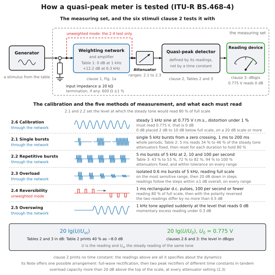
verify_quasi_peak_dynamics builds the clause 2.1 and 2.2 stimuli exactly as
specified: a 5 kHz sine starting at a zero crossing and lasting an integral
number of full periods, through the weighting network, and reads each against
the same chain’s steady reading.
from phonometry import broadcast
report = broadcast.verify_quasi_peak_dynamics(48000.0)print(report.passes, round(report.worst_margin_db, 3))   # True 0.259row = report.stimuli[0]print(row["stimulus"], round(row["reading_percent"], 2))       # 1 ms 16.94
All eleven windows are met at 32, 44.1, 48, 96 and 192 kHz. The worst margin is 0.259 dB, at the 100 bursts per second cell whose upper limit is the physical ceiling. Between those five rates no reading moves by more than 0.080 dB, or 4.2 % of its own window, which is why the peak-follower worry about reading the largest sample rather than the largest value of the waveform does not bite here: the 1.41 ms charge spans fourteen half-periods of the rectified 5 kHz carrier, so the ripple is long gone before any maximum is taken.
deviation_db is also reported, against the reference column, and the
report calls it what it is: a self-imposed regression bound, not conformance.
The worst is 0.140 dB, at 10 bursts per second. The reference row is printed
to two significant figures on nine of the eleven cells, so its own quantum is
0.027 to 0.108 dB, and nothing tighter than that would mean anything.
Four further clauses are computable and pass by construction rather than by measurement, because rectification, first-order recursions and a maximum are positively homogeneous and cannot overshoot a monotone step: clause 2.1’s two attenuator variants, clause 2.3’s ±1 dB over 20 dB of 0.6 ms bursts, clause 2.4’s 0.5 dB reversibility (, so the difference is exactly zero) and clause 2.5’s 0.3 dB overswing cap. The rest of clauses 2.3, 2.6 and 2.7 has nothing to compute at all: overload capacity above full scale, the law of a logarithmic stage, a calibrated scale range of at least 20 dB, an input impedance of at least 20 kΩ and a 600 Ω termination are instrument hardware. So is “80 % of full scale”, which constrains where a real needle sits during the test rather than the quantity, which is why this library models no full scale at all.
How the measurement goes
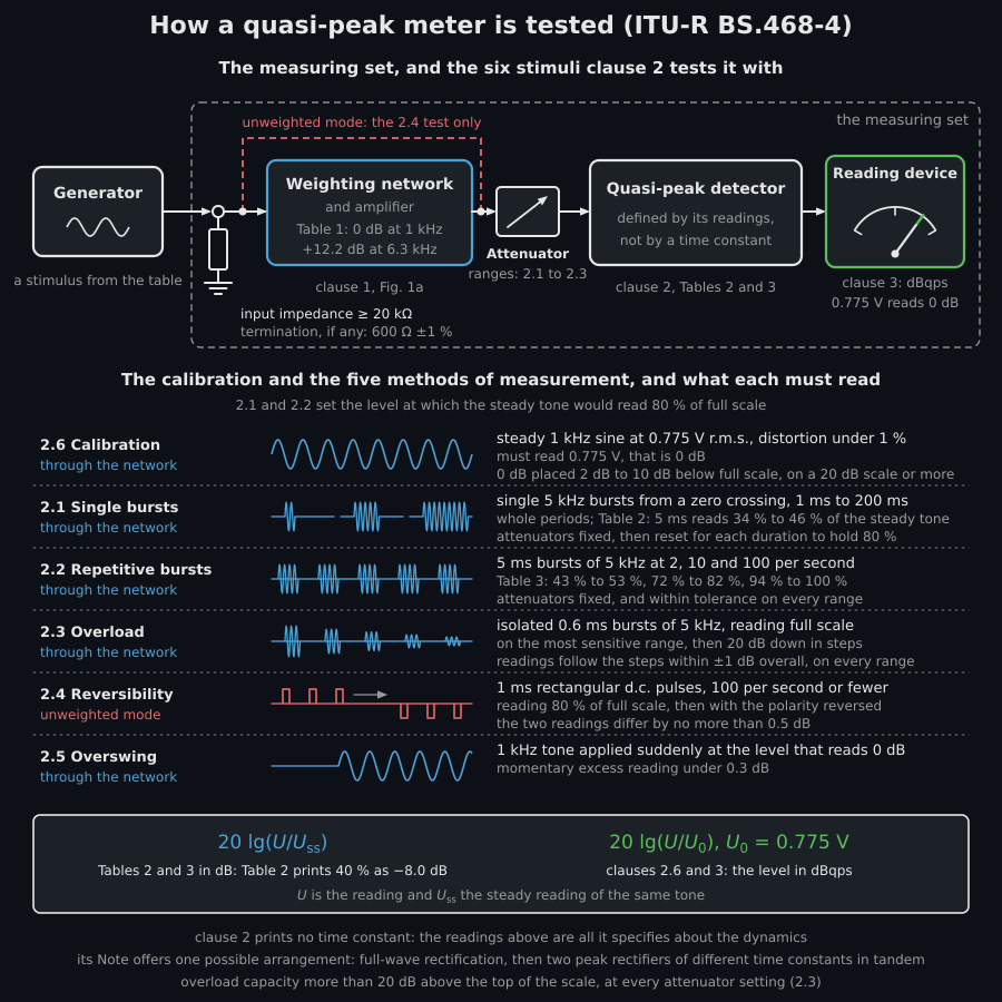
Section titled “How the measurement goes”Calibrate first, to 2.6: a steady 1 kHz sine of 0.775 V r.m.s., with under 1 % total harmonic distortion, must read 0.775 V, 0 dB. The input impedance should be at least 20 kΩ, and 600 Ω ±1 % where a termination is provided. Every test but 2.4 runs through the weighting network. For 2.1, set the level at which a steady 5 kHz tone would read 80 % of full scale and apply single bursts of whole periods from a zero crossing, one for each duration of Table 2, read once with the attenuators untouched and once reset for each duration to hold the reading near 80 %. For 2.2, apply 5 ms bursts at 2, 10 and 100 per second at that level, attenuators untouched, and check Table 3 on every range. For 2.3, bring isolated 0.6 ms bursts to full scale on the most sensitive range and step them down 20 dB in all: the readings have to follow within ±1 dB overall, range by range. For 2.4, switch to the unweighted mode, apply 1 ms rectangular d.c. pulses, 100 per second or fewer, reading 80 % of full scale, and reverse their polarity: the readings may differ by 0.5 dB at most. For 2.5, switch the 1 kHz tone on suddenly at 0 dB: the momentary excess reading must stay under 0.3 dB. Noise read on an instrument that passes is expressed in dBqps.
6. What no oracle can check
Section titled “6. What no oracle can check”The tables use one carrier, one waveform, one amplitude, eight durations and three repetition rates, and that is the whole specification of the detector. There is no reference implementation, no tabulated impulse response and no worked example in BS.468-4, in IEC 60268-1:1985 Appendix A or in either 1988 amendment. So:
- The response to noise is unverifiable, and noise is the instrument’s entire purpose. Two conforming detectors will disagree on noise, on speech and on programme material by an amount nothing in the document bounds. How much is measurable from this side. Sampling the three time constants inside their identified ranges and keeping only the sets that meet all eleven windows gives 243 conforming detectors, and on a one-sample click they read 4.61 dB apart, on a 1 ms pulse 4.61 dB and on a single-cycle 5 kHz burst 4.55 dB. That is more than the widest window the tables draw (4.00 dB) and eight times the narrowest (0.54 dB). On white noise the same 243 spread 0.71 dB, and on a steady 1 kHz tone 0.00 dB, which is the clause 2.6 calibration doing exactly what it promises: it is transients the tables fail to pin, which is where a quasi-peak meter differs from an r.m.s. one in the first place. The record has to be long enough for the needle to finish rising before any of this is read, or the slow sets are caught mid-climb and the spread measured is the truncation instead.
- So is the relationship between a dB(468) quasi-peak figure and a dB(A) r.m.s. one for any real signal. The rule of thumb that a microphone’s BS.468 self-noise figure comes out about 10 dB above its A-weighted one is a statement about typical microphone noise spectra, not about either standard.
- So is everything outside the tabulated stimuli: bursts shorter than 0.6 ms or longer than 200 ms, carriers other than 5 kHz, repetition rates other than 2, 10 and 100 per second, and anything that is not a gated sine.
There is no .report() fiche for this measurement, and that is a decision
about the standard rather than about effort. BS.468-4 prescribes no report
format, no declaration form, no worked example and no reporting clause beyond
clause 3’s one sentence naming the unit. A conformity sheet in an accredited
format would attest this library’s own filter, on a page carrying a
standard-basis line, with eleven numbers produced by ballistics this project
fitted. The conformity evidence is real and it is published, in
docs/CONFORMANCE.md, through
verify_quasi_peak_dynamics.
What this guide covers
Section titled “What this guide covers”Covered
ITU-R BS.468-4 clause 2: the quasi-peak detector, its eleven Table 2 and Table 3 acceptance windows, and the clause 2.6 calibration that fixes the dBqps scale.
quasi_peak_meterruns the detector,QuasiPeakResultcarries the reading and the needle,BS468_BALLISTICSholds the three fitted time scales andverify_quasi_peak_dynamicschecks all eleven windows at any sample rate. Clauses 2.1, 2.3, 2.4 and 2.5 are exercised in the test suite as properties of the chain. Clause 1’s weighting network isweighting_filter(curve="468").Not covered
Annex 2’s unweighted response is a graphical tolerance template offered “for guidance” and explicitly outside the scope of the Recommendation; it has no table, no formula and no filter order, so nothing here implements it. The Annex 1 constant-resistance realization is an alternative hardware build of the same response, with coupled windings whose coupling coefficients the figure does not give, and adds nothing a software implementation needs. The instrument requirements of clauses 2.3, 2.6 and 2.7 (overload capacity, the law of a logarithmic stage, the calibrated scale range, input impedance and the 600 Ω termination) are hardware and are not modelled. There is no
.report()fiche, for the reason in section 6.
Standards
Section titled “Standards”ITU-R BS.468-4 (1970-1974-1978-1982-1986, with 2002 editorial amendments), Measurement of audio-frequency noise voltage level in sound broadcasting: clause 2’s quasi-peak method, the Table 2 single-burst and Table 3 repetitive-burst acceptance windows, the clause 2.6 calibration at 1 kHz and 0.775 V r.m.s., and clause 3’s unit dBqps. Clause 2 prints no time constant, so the dynamics of any conforming detector are a design choice inside those eleven windows; the three time scales this library uses are a fit, identified by the tables only to within a factor of 1.61 to 2.09, and least of all in the reading device.
References
Section titled “References”- Audio Engineering Society. (2015). AES standard method for digital audio engineering - Measurement of digital audio equipment (AES17-2015). Clause 5.2.7 uses the same curve shifted by -5.63 dB with an r.m.s. detector and renames the result CCIR-RMS, which is precisely not the measurement on this page.
- International Electrotechnical Commission. (1985). Sound system equipment - Part 1: General (IEC 60268-1:1985, Appendix A (with Amendment 1:1988)). The same network and the same meter, as Table AI, Fig. A1 and Tables AII and AIII. Two of its cells are misprints and one of those was corrected by the amendment; see docs/ERRATA.md.
- International Telecommunication Union. (2002). Measurement of audio-frequency noise voltage level in sound broadcasting (Recommendation ITU-R BS.468-4). Clause 1 and Fig. 1a for the weighting network, clause 2 for the quasi-peak detector (the Table 2 and Table 3 acceptance windows, the clause 2.6 calibration) and clause 3 for the unit dBqps.