Hydrodynamic Valve Noise (IEC 60534-8-4)

Water is compressible enough to carry sound at 1 400 m/s and far too stiff to choke the way a gas does, so a control valve on a water line cannot build the shock cells that the aerodynamic part spends five regimes on. It makes noise two ways instead, and the whole of IEC 60534-8-4 is the sum of them: turbulence in the jet leaving the vena contracta, and cavitation, once the pressure there falls low enough for the liquid to flash to vapour and the bubbles to collapse again downstream.

The difference between the two is not a matter of degree. Turbulent noise follows the jet velocity gently; cavitation arrives at a threshold and then climbs as a fifth power. Everything on this page turns on where the operating point sits with respect to that threshold.

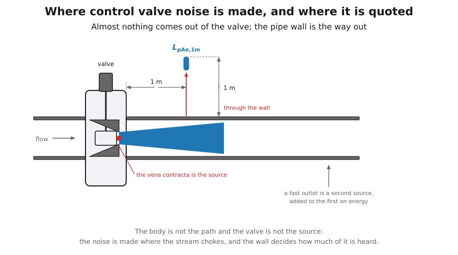
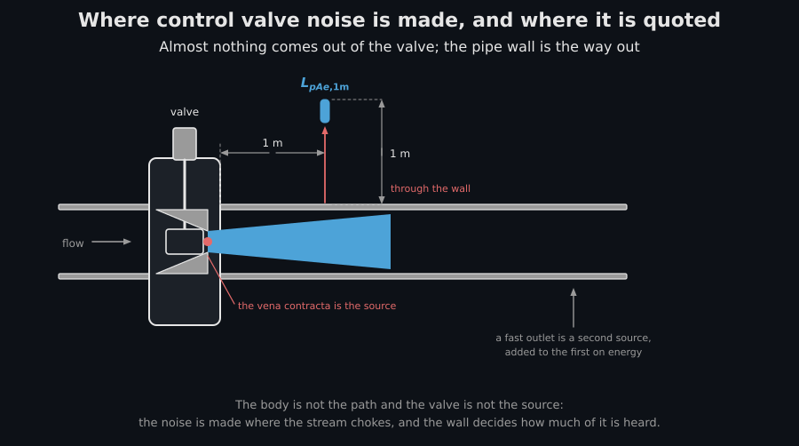
The liquid case changes the source and not the geometry: the bubbles collapse where the jet is, and the level is quoted at the same metre.

Two ratios decide the regime. The first is the differential pressure ratio, Equation (1), which says how far towards flashing this operating point is:

The second is the characteristic pressure ratio $x_{Fz}$: the value of $x_F$ at which cavitation first becomes audible on this valve. It is a property of the valve, measured to IEC 60534-8-2, and 4.2 offers Equation (3a) only as an estimate for when no measurement exists. Equation (3c) then moves it from the 6 × 10⁵ Pa the estimate is drawn at to the working inlet pressure.

from phonometry import noise_control

x_f = noise_control.differential_pressure_ratio(
    inlet_pressure_pa=1.0e6, outlet_pressure_pa=6.5e5, vapour_pressure_pa=2.32e3
)
print(round(x_f, 4))                                    # 0.3508

x_fz = noise_control.incipient_cavitation_ratio(90.0, 0.42, 0.92)
print(round(x_fz, 4))                                   # 0.2543  at 6e5 Pa
print(round(noise_control.corrected_incipient_ratio(x_fz, 1.0e6), 4))
#                                                       # 0.2386  at 10 bar

This valve is past its threshold, so it cavitates. A multihole trim of the same capacity would not be: Equation (3b) answers on the hole geometry rather than on the capacity, and a hundred and twenty holes of three millimetres push the threshold up by half. The comparison has to be made against the corrected value, which is the half of it a reader is most likely to skip.

holes = noise_control.multihole_incipient_cavitation_ratio(120, 0.003, 0.92)
print(round(holes, 4))                                  # 0.3941  at 6e5 Pa
print(round(noise_control.corrected_incipient_ratio(holes, 1.0e6), 4))
#                                                       # 0.3698  still above x_F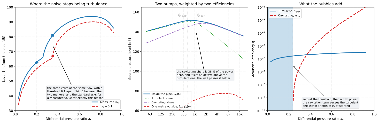

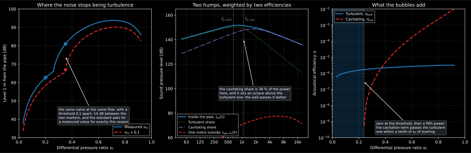
The left panel is Annex A’s own Figure A.1: the same valve at the same flow, with a characteristic pressure ratio 0,1 apart, and 14 dB between the two markers at $x_F=0,35$.

That 14 dB is the reason 4.2 warns that a prediction built on the estimate “can create uncertainties”. The estimate is not a small correction to the answer; on a cavitating valve it is the answer.

The source half of the method is short. The differential of Equation (2) is capped at the choking point, Equation (5) turns it into a jet velocity and Equation (6) into the stream power the valve dissipates:

choked = noise_control.cavitation_differential(
    inlet_pressure_pa=1.0e6,
    outlet_pressure_pa=6.5e5,
    vapour_pressure_pa=2.32e3,
    pressure_recovery=0.92,
)
speed = noise_control.vena_contracta_velocity(choked, 997.0, 0.92)
power = noise_control.mechanical_stream_power(40.0, speed, 0.92)
print(round(speed, 3), round(power, 1))                 # 28.801 14042.1

Then two efficiencies say what fraction of those fourteen kilowatts leaves as sound. Equation (8) makes the turbulent one linear in the jet Mach number, reaching $10^{-4}$ only when the jet reaches the speed of sound in the liquid, which for water is 1 400 m/s and never happens in a control valve:

Equation (9) is the other one, and it is worth reading factor by factor:

Three of those factors do all the work. $(x_F-x_{Fzp1}{)}^{1,5}$ starts the term at exactly zero on the threshold, so the two regimes meet without a step. $(x_F/x_{Fzp1}{)}^5$ then makes it climb almost vertically. And $(1-x_F{)}^{-0,5}$ sends it towards infinity as the valve approaches flashing, which is where the method stops.

turbulent = noise_control.turbulent_efficiency(speed, 1400.0)
cavitating = noise_control.cavitation_efficiency(
    turbulent=turbulent,
    differential=3.5e5,
    choked_differential=choked,
    pressure_ratio=0.3508,
    corrected_ratio=0.2386,
)
print(f"{turbulent:.3e} {cavitating:.3e}")              # 2.057e-06 1.242e-06

Just past the threshold the cavitation term is already comparable with the turbulent one, and Equation (7b) adds them before Table 2’s acoustic power ratio $r_W$ takes the share that is radiated into the pipe rather than lost in the body: a quarter for every globe and rotary valve, a half for the butterflies, one for an expander.

res = noise_control.valve_hydrodynamic_noise(
    noise_control.LiquidStream(
        mass_flow=40.0,                # kg/s
        inlet_pressure_pa=1.0e6,          # Pa, absolute
        outlet_pressure_pa=6.5e5,
        vapour_pressure_pa=2.32e3,
        density=997.0,                 # kg/m3
        speed_of_sound=1400.0,            # m/s
    ),
    noise_control.LiquidTrim(
        flow_coefficient=90.0,         # C_v
        style_modifier=0.42,           # F_d, from IEC 60534-8-3
        pressure_recovery=0.92,        # F_L
        incipient_ratio=x_fz,          # x_Fz, at 6e5 Pa
        power_ratio=0.25,              # r_W, Table 2
        valve_diameter_m=0.1,            # m
        seat_diameter_m=0.1,             # m
    ),
    noise_control.LiquidPipe(
        internal_diameter_m=0.1071,      # m
        wall_thickness=0.0036,         # m
        density=7800.0,                # kg/m3, steel
    ),
)
print(res.regime)                                       # cavitating
print(round(res.sound_power, 5), "W")                   # 0.01158 W
print(round(res.internal_level, 3), "dB")               # 156.543 dB
print(round(res.turbulent_peak, 2), round(res.cavitation_peak, 2))
#                                                       # 654.35 1088.94
print(round(res.external_level, 1), "dB at 1 m")        # 81.0 dB at 1 m

Every one of those is a printed cell of Annex A’s Table A.1. The same call on the first column, 30 kg/s into 8 bar, stays turbulent and answers 62,7 dB; the third column is the second one again with $x_{Fz}$ shifted by 0,1, and answers 66,9 dB.

The two peak frequencies are Equations (11) and (13), and (13) is the surprising one: on the threshold the cavitating peak is six times the turbulent peak, and it falls from there as the valve is opened further into cavitation, because the bubbles grow larger and take longer to collapse. Just past onset, cavitation is a hiss; deep into it, a rumble.

Inside the pipe this valve runs at 156 dB. What makes the outside habitable is the wall, and the standard anchors its transmission loss at the ring frequency, Equation (14), where one wavelength in the wall material wraps exactly once around the circumference:

print(round(res.pipe_ring_frequency, 1), "Hz")          # 14860.4 Hz
print(round(res.reference_transmission_loss, 2), "dB")  # -44.71 dB
print(round(res.transmission_loss, 2), "dB")            # -62.86 dB

Both terms of Equation (15) are printed with a minus sign, so the transmission loss of this method is a negative number that is added all the way to the end. Away from the ring frequency Equations (16b) and (22b) only make it worse, and the peak frequencies of a control valve are more than a decade below the ring frequency of its pipe, which is where the other 18 dB of this valve’s loss come from: Equation (16b) costs 27 dB at the turbulent peak, and Equation (17) hands 9 of them back because the valve cavitates.

Band by band, 5.4 spreads the internal level with Equations (20a) and (20b) and gives the wall a frequency-dependent loss with Equation (22a):

import numpy as np

band = int(np.argmin(np.abs(res.frequencies - 8000.0)))
print(round(float(res.band_internal_level[band]), 1))     # 141.9
print(round(float(res.band_transmission_loss[band]), 2))  # -51.76
print(round(float(res.band_external_level[band]), 1))     # 77.4

Those three are printed in Table A.1 as 141,9 dB, 51,76 dB and 77,4 dB. The middle one is printed without its minus sign, and it cannot be: its own two inputs, $-44,71$ and $-7,053$ dB, sum to $-51,763$, and the row below only reproduces its printed 77,4 dB with the negative value. The errata register records it, along with three intermediates of the same table that its own equations do not reproduce.

Equation (12), the Strouhal number that places the turbulent peak, appears twice in the document and not identically. Clause 5.1 prints a leading 0,02 and no valve style modifier; Table A.1 prints 0,036 and a factor $F_d^{0,75}$. Both are on the page, and they are not the same function of the valve.

form = dict(
    flow_coefficient=90.0,
    style_modifier=0.42,
    pressure_recovery=0.92,
    corrected_ratio=0.2386,
    valve_diameter_m=0.1,
    seat_diameter_m=0.1,
    inlet_pressure_pa=1.0e6,
    vapour_pressure_pa=2.32e3,
)
print(round(noise_control.jet_strouhal_number(**form, form="annex"), 3))   # 0.399
print(round(noise_control.jet_strouhal_number(**form, form="clause"), 3))  # 0.425

Only the annex form reproduces the annex’s own printed $N_{Str}=0,399$, so it is the default here and the clause form is one keyword away. For this valve the two differ by 6 %; for a single-port valve with $F_d=1$ the annex form is 80 % above the clause one, which is five sixths of an octave in the peak frequency and a few decibels through the transmission loss.

Clause 6 is the same method with per-stage inputs. Each stage takes a share of the differential in inverse proportion to the square of its own flow coefficient, which is the series law $1/C^2={\sum }_{i}1/C_i^2$:

stages = noise_control.stage_conditions(
    inlet_pressure_pa=1.0e6,
    outlet_pressure_pa=4.0e5,
    vapour_pressure_pa=2.32e3,
    stage_coefficients=[130.0, 160.0, 199.1],
    flow_coefficient=90.0,
)
for stage in stages:
    print(round(stage.inlet_pressure_pa), round(stage.pressure_ratio, 3))
# 1000000 0.288
# 712426 0.267
# 522582 0.236

print(round(noise_control.combine_stage_levels(78.0, 74.0, 71.0), 1))   # 80.0

Those three coefficients increase along the flow, which is the device of Figure 2: most of the pressure is taken in the first stages and the last one is left working at a differential small enough not to cavitate. 6.3.2 then calculates only that last stage, because the sound the earlier ones make is absorbed inside the trim before it reaches the pipe, and it caps the differential at the last stage’s own cavitation threshold rather than at the choking point:

print(noise_control.last_stage_differential(
    inlet_pressure_pa=6.0e5,
    outlet_pressure_pa=4.0e5,
    vapour_pressure_pa=2.32e3,
    corrected_ratio=0.30,
))                                                      # 179304.0

print(noise_control.uniform_passage_style_modifier(16))            # 0.25
print(round(noise_control.last_stage_seat_diameter_mm(45.0), 1))   # 37.7

The last of those carries its unit in its name for a reason. The formula it implements is the one display formula in the standard with no equation number, $d_o=5,2\sqrt{N_{34}{C}_n}$, and Clause 3 declares $d_o$ in metres, which for any real last stage it cannot be: 37,7 of anything is millimetres. Divide by a thousand before handing it to Equation (12).

• Covered

  IEC 60534-8-4:2005, Clauses 4, 5 and 6, against all three worked examples of Annex A. The preliminary calculations of Clause 4: the differential pressure ratio of Equation (1), the capped differential of Equation (2), the characteristic pressure ratio of Equations (3a) and (3b) with the inlet correction of (3c), the jet diameter of (4), the vena contracta velocity of (5) and the stream power of (6). The noise prediction of Clause 5: the two acoustical efficiencies of Equations (8) and (9) and the sound power of (7a) and (7b), the internal level at the pipe wall of (10), the Strouhal number and both peak frequencies of (11) to (13), the ring frequency and transmission loss of (14) to (17) with the floor of the NOTE, the external level of (18a) and (18b), and the whole frequency route of 5.4 in bands. And Clause 6 for a multistage trim: the stage pressures and ratios of Equations (23a) to (26), the energy sum of (27), and the last-stage differential, style modifier and seat diameter of 6.3.2.

• Not covered yet

  The measurement of $x_{Fz}$ itself, which is the laboratory procedure of IEC 60534-8-2 and not a calculation, and the typical curves of Figures 4 to 9 that stand in for it: this page takes the value as an argument. Flashing, the regime past $x_F=1$ where the liquid leaves the valve as vapour, which the method excludes and the library refuses rather than extrapolates.

References

Section titled “References”- International Electrotechnical Commission. (2005). Industrial-process control valves — Part 8-4: Noise considerations — Prediction of noise generated by hydrodynamic flow (IEC 60534-8-4:2005). The whole of this page: Clauses 4, 5 and 6 with their Tables 1 and 2, and the three worked examples of Annex A.
- International Electrotechnical Commission. (2010). Industrial-process control valves — Part 8-3: Noise considerations — Control valve aerodynamic noise prediction method (IEC 60534-8-3:2010). Where the valve style modifier and the jet diameter come from: 4.3 and 4.4 of the hydrodynamic part send the reader there rather than printing them again.
- International Electrotechnical Commission. (2014). Electroacoustics — Octave-band and fractional-octave-band filters — Part 1: Specifications (IEC 61260-1:2014). The one-third-octave bands from 50 Hz to 20 kHz that 5.4.1 names and every spectrum on this page is carried on.