Swept-sine distortion and phase utilities

A single exponential sine sweep characterises the linear response and every harmonic distortion order of a weakly nonlinear system at once. After deconvolution, the distortion products of order $n$ pack into separate impulse responses that precede the linear response by the fixed advance (Farina 2000)

$$\Delta t_n=T\frac{\ln n}{\ln (f_2/f_1)}=L\ln n,L=\frac{T}{\ln (f_2/f_1)},$$

so windowing each arrival yields the higher harmonic frequency responses $H_1(f),H_2(f),\dots ,H_N(f)$ and, from them, the total harmonic distortion as a function of the excitation frequency with one sweep instead of a tone-by-tone stepping. This page covers that separation in phonometry.electroacoustics, with the phase-coherent synchronized sweep of Novak, Lotton & Simon (2015) as the default, and the companion phase utilities in phonometry.signals: minimum phase from $|H|$, group delay and excess phase.

1. One sweep, every harmonic

For an exponential sweep the instantaneous frequency rises as $f(t)=f_1{e}^{t/L}$, so the moment the excitation passes $f$, the n-th harmonic distortion product appears at $nf$: exactly where the sweep itself will be $L\ln (n)$ seconds later. Deconvolving the recording against the sweep therefore time-compresses each order into its own impulse response, $L\ln (n)$ before the linear one. swept_sine_distortion windows each arrival (with the exact fractional-sample alignment), Fourier transforms it into $H_n(f)$, and reads the distortion of order $n$ at excitation frequency $f$ from $|H_n(nf)|$:

$$\mathrm{THD}(f)=\frac{\sqrt{{\sum }_{n\ge 2}|H_n(nf){|}^2}}{|H_1(f)|}.$$

The chain is exactly the sketch below: play the sweep, record, convolve with the inverse filter, and the harmonics land ahead of the linear response by their fixed advances.

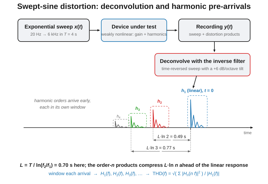
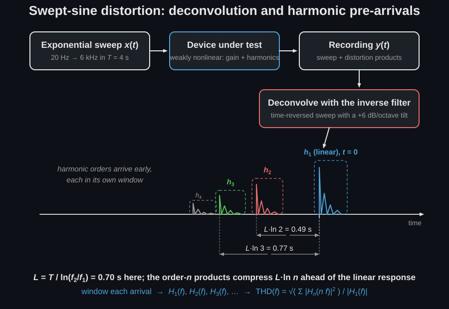
The advances are fixed by the sweep alone — $L=T/\ln (f_2/f_1)=0.70$ s here — and not by the device, which is why the same windows work for any weakly non-linear system and why lengthening the sweep is what buys separation.

import numpy as np
from phonometry import swept_sine_distortion, synchronized_sweep_signal

fs, f1, f2, seconds = 48000, 20.0, 6000.0, 4.0
x = synchronized_sweep_signal(fs, f1, f2, seconds)   # play this...
# ... record the device response into `y` (include the decay tail) ...
res = swept_sine_distortion(y, fs, f1, f2, seconds, n_harmonics=3)

res.harmonic_responses    # complex H1..H3 on res.frequencies
res.thd, res.thd_frequencies
res.distortion_ratios     # |Hn(n f)| / |H1(f)| per order
res.plot()                # |Hn| magnitudes + THD(f)

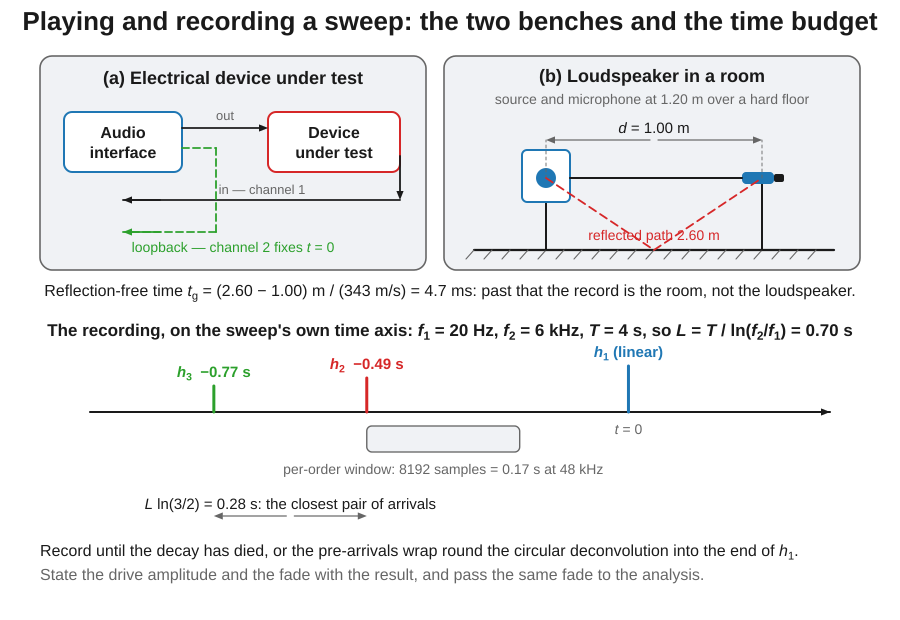
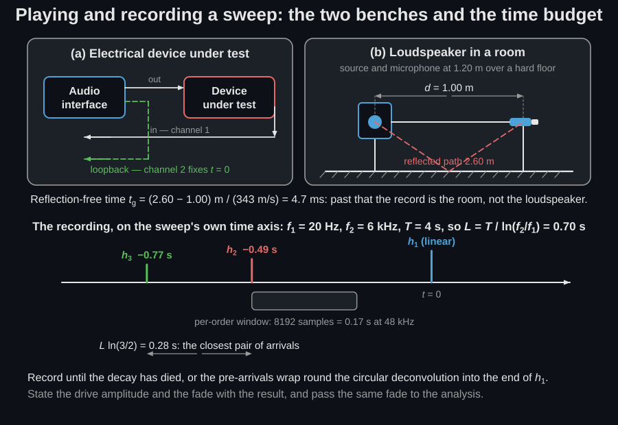
1.1 Playing and recording it

A THD(f) curve is a property of the device at one drive level, so it has to be published with that level — and, for an acoustic measurement, with the sound pressure level it produced at the microphone. The same loudspeaker measured 6 dB louder returns a curve several decibels higher and differently shaped, because the mechanisms that dominate change with excursion. Choose the level between two walls: high enough that the harmonics stand clear of the background, because the deconvolution’s processing gain helps the linear response far more than it helps the pre-arrivals, and low enough that neither the device nor any converter in the chain clips — a clipped record manufactures exactly the odd-order harmonics being measured, in every window. Note also that a sweep has a much lower crest factor than a tone burst, so at equal peak amplitude it delivers more energy and pushes a device harder than a tone test at the same nominal level.

Four things must be set before the first take:

import numpy as np

# `synchronized_sweep_signal` and `swept_sine_distortion` as imported above.
x = synchronized_sweep_signal(fs, f1, f2, seconds, amplitude=0.5, fade=0.02)
# ... play x, record y, and keep recording until the decay has died ...
res = swept_sine_distortion(y, fs, f1, f2, seconds, n_harmonics=3,
                            amplitude=0.5, fade=0.02)

• amplitude is the reference the returned $H_1$ and every ratio are computed against, so it must be the level actually played, and the same value has to reach both calls: the analysis defaults to 1.0, so a sweep generated at 0.5 and analysed at the default returns a gain 6 dB low.
• fade applies a short half-Hann taper at both ends. It is 0 by default because the analysis is exact on the unfaded sweep, but an unfaded sweep starts and ends on a full-amplitude discontinuity that clicks through a real amplifier and loudspeaker and smears energy across the whole harmonic time axis. The same value must be passed to the analysis, or the deconvolution is mismatched; 20 ms reshapes only the extreme band edges.
• Clipping. Check every stage, not just the converter: the point of the measurement is destroyed by any element that clips before the one under test.
• The tail. Record the sweep plus its full decay, or the harmonic pre-arrivals wrap round the circular deconvolution into the end of the linear response.

Two failure modes are silent rather than obvious. The method assumes the system does not change during the sweep, so a running fan, a person moving, a warming voice coil or a drifting room temperature decorrelates the later part of the sweep from the earlier part and shows up as a raised noise floor around the harmonic arrivals rather than as an evident failure — which is why long measurements are averaged rather than lengthened indefinitely. And any impulsive event in the recording is spread by the deconvolution across the whole time axis, landing inside the harmonic windows where it is read as distortion: one loud click can invent several percent of THD, so repeat the measurement rather than trying to gate it out. Finally, the residual noise floor of the deconvolution is the floor of the THD(f) curve — a 60 dB signal-to-noise capture cannot show a 0.05 % harmonic however the windows are placed — so report the measured noise floor beside the curve.

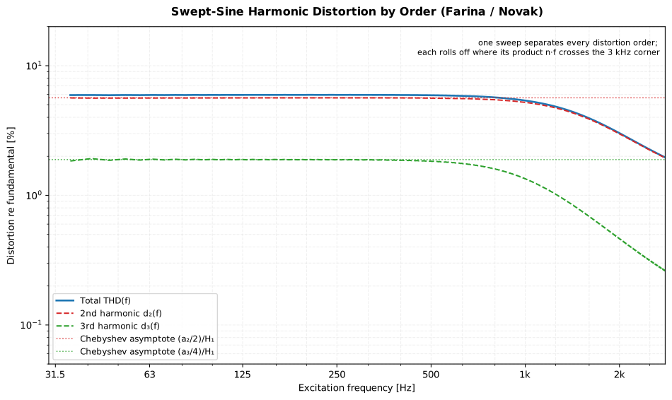
The flat low-frequency plateaus are the Chebyshev levels $(a_2/2)/H_1$ and $(a_3/4)/H_1$ of the memoryless polynomial, and each order bends down where its own product $nf$ crosses the 3 kHz post-filter — so the knees are at 1.5 kHz for $d_2$ and 1 kHz for $d_3$, on the excitation axis. That is the same oracle the conformance tests pin.

Show the code for this figure

import matplotlib.pyplot as plt
import numpy as np
from scipy import signal as sp_signal
from phonometry import swept_sine_distortion, synchronized_sweep_signal

fs, f1, f2, seconds = 48000, 20.0, 6000.0, 4.0
a2, a3 = 0.12, 0.08
x = synchronized_sweep_signal(fs, f1, f2, seconds)
b, a = sp_signal.butter(2, 3000.0, fs=fs)             # 3 kHz post-filter
y = sp_signal.lfilter(b, a, x + a2 * x**2 + a3 * x**3)
res = swept_sine_distortion(y, fs, f1, f2, seconds, n_harmonics=3)

h1 = 1.0 + 3.0 * a3 / 4.0                              # Chebyshev gain
fig, ax = plt.subplots(figsize=(10, 6))
ax.loglog(res.thd_frequencies, 100.0 * res.thd, label="Total THD(f)")
ax.loglog(res.thd_frequencies, 100.0 * res.distortion_ratios[0],
          ls="--", label="2nd harmonic d2(f)")
ax.loglog(res.thd_frequencies, 100.0 * res.distortion_ratios[1],
          ls="--", label="3rd harmonic d3(f)")
ax.axhline(100.0 * (a2 / 2.0) / h1, ls=":",
           label="Chebyshev asymptote (a2/2)/H1")
ax.axhline(100.0 * (a3 / 4.0) / h1, ls=":",
           label="Chebyshev asymptote (a3/4)/H1")
ax.set_xlabel("Excitation frequency [Hz]")
ax.set_ylabel("Distortion re fundamental [%]")
ax.legend()
plt.show()

The oracle behind the implementation is the memoryless polynomial: driving $y=x+a_2{x}^2+a_3{x}^3$ with a unit sweep must return, by the Chebyshev identities, $|H_1|=1+3a_3/4$, $|H_2|=a_2/2$ (phase $-\pi /2$), $|H_3|=a_3/4$ (phase $\pi$) and $\mathrm{THD}=\sqrt{(a_2/2{)}^2+(a_3/4{)}^2}/(1+3a_3/4)$. The test and conformance suites pin all four, and the same THD measured tone by tone with phonometry.thd agrees to 0.1 %.

What the method exists to produce, though, is not the scalar ratios — a stepped tone sweep gives those too — but the set of harmonic transfer functions. Each $H_n$ is a full frequency response over its own band $[n{f}_1,n{f}_2]$:

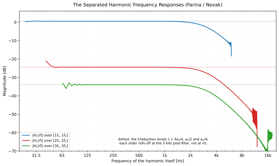
Each order is a response, not a number, and here they are plotted against the frequency of the harmonic itself: all three roll off at the same 3 kHz, because the post-filter acts on the product and not on the excitation. The dotted lines are the Chebyshev levels. res.plot() draws these magnitudes together with the THD(f) panel above.

Show the code for this figure

import matplotlib.pyplot as plt
import numpy as np
from scipy import signal as sp_signal

# `swept_sine_distortion` and `synchronized_sweep_signal` as imported above.
fs, f1, f2, seconds = 48000, 20.0, 6000.0, 4.0
a2, a3 = 0.12, 0.08
x = synchronized_sweep_signal(fs, f1, f2, seconds)
b, a = sp_signal.butter(2, 3000.0, fs=fs)
y = sp_signal.lfilter(b, a, x + a2 * x**2 + a3 * x**3)
res = swept_sine_distortion(y, fs, f1, f2, seconds, n_harmonics=3)

for k in range(3):
    mag = np.abs(np.asarray(res.harmonic_responses[k]))
    plt.semilogx(res.frequencies, 20 * np.log10(np.maximum(mag, 1e-9)))
plt.show()

Reading a real device. On a measured driver the curve has a shape worth recognising: distortion rising steeply below the fundamental resonance, where excursion grows as the response falls; a local peak wherever a resonance is being driven hard; and a floor of a fraction of a percent through the mid band at moderate drive. Separating the orders is what makes the curve diagnostic: a dominant second harmonic is asymmetry — a voice coil not centred in the gap, a suspension stiffer in one direction than the other — while a dominant third is symmetric limiting, the suspension or the magnetic gap running out at both extremes, and the two call for different fixes. For scale, below about 1 % through the mid band is unremarkable for a direct radiator at conversational levels, 10 % is the conventional marker for the excursion limit that defines a driver’s usable low-frequency end, and any amplifier reaching 1 % below clipping is broken. Remember that the abscissa is the excitation frequency: a feature at 100 Hz on the $d_2$ trace is energy radiated at 200 Hz, which is where it will be heard.

2. The synchronized sweep (Novak et al. 2015)

Windowing separates the harmonic magnitudes with any exponential sweep, but the phases of $H_2\dots H_N$ are only meaningful if delaying the sweep by $L\ln (n)$ is exactly equivalent to generating its n-th harmonic. That holds only for

$$x(t)=\sin \left[2\pi f_{1}L{e}^{t/L}\right],L=\frac{1}{f_1}\mathrm{round}\left(\frac{f_1\tilde{T}}{\ln (f_2/f_1)}\right),$$

the synchronized swept-sine: the rounding makes $f_{1}L$ an integer, so the sweep starts at zero phase and every harmonic copy lines up. synchronized_sweep_signal generates it (the duration is quantized slightly; when $f_2/f_1$ is an integer the sweep also ends at zero phase), and swept_sine_distortion(..., method="synchronized"), the default, deconvolves with the closed-form spectrum of the inverse filter,

$$\tilde{X}(f)=2\sqrt{f/L}{e}^{-j2\pi fL(1-\ln (f/f_1))+j\pi /4},$$

rather than an FFT of the signal. Besides being exact, the analytic deconvolution extends the usable band of each $H_n$ to $[n{f}_1,n{f}_2]$ (Novak et al., Fig. 6): the second harmonic of a 6 kHz sweep is measured up to 12 kHz.

Two practical notes from the paper are built in: the recording mean is subtracted by default (remove_dc=True; a DC offset otherwise leaks a scaled inverse filter into the impulse response), and the non-integer part of each arrival $L\ln (n)f_s$ is removed in the frequency domain, so the harmonic phases carry no residual sub-sample skew.

3. Analysing classical exponential-sweep (ESS) recordings (method="farina")

Recordings made with the plain exponential sine sweep (ESS) of phonometry.sweep_signal (the ISO 18233 excitation used by impulse_response) are analysed with method="farina": the same windowing over the time-reversed, amplitude-compensated inverse filter of Farina (2000). The harmonic magnitudes and the THD are correct (the Chebyshev oracle passes identically), but the sweep’s -1 phase term breaks the time-shift equivalence, so the phases of $H_2\dots H_N$ depend on the excitation and should be ignored; the band of every $H_n$ is also capped at $f_2$ by the inverse filter.

from phonometry import sweep_signal, swept_sine_distortion

x = sweep_signal(fs, f1, f2, seconds)          # the ISO 18233 ESS
res = swept_sine_distortion(y, fs, f1, f2, seconds, method="farina")
res.plot()   # same |Hn| + THD(f) panels as the synchronized method (needs matplotlib)

The result is the same plottable SweptSineDistortionResult as the synchronized method, so the |Hn| and THD(f) panels of the section-1 figure read identically; only the harmonic phases (and the top of each order’s band) differ between the two methods. Both differences are visible on one recording:

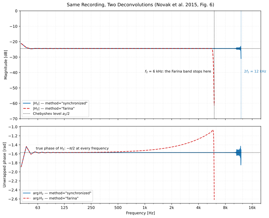
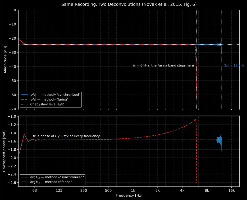
Same recording, same magnitudes, two differences. The synchronized deconvolution measures $H_2$ up to $2f_2$; the Farina inverse filter stops it at $f_2$. And on a device whose true $H_2$ phase is exactly $-\pi /2$ at every frequency (the memoryless cubic of the oracle), only the synchronized phase reproduces it — which is why method="farina" returns phases that must be discarded rather than read.

Show the code for this figure

import matplotlib.pyplot as plt
import numpy as np

# `synchronized_sweep_signal` and `swept_sine_distortion` as imported above.
x = synchronized_sweep_signal(48000, 20.0, 6000.0, 4.0)
y = x + 0.12 * x**2 + 0.08 * x**3            # the memoryless oracle
actual = len(x) / 48000                       # the generator quantizes T
for method in ("synchronized", "farina"):
    res = swept_sine_distortion(y, 48000, 20.0, 6000.0, actual,
                                n_harmonics=3, method=method)
    plt.semilogx(res.frequencies,
                 np.unwrap(np.angle(np.asarray(res.harmonic_responses[1]))))
plt.show()

4. Sizing the sweep

Before recording anything, three numbers have to agree: the sweep duration $T$, the number of harmonic orders $N$ and the top frequency $f_2$. The rules below govern both methods.

• The window against the arrival spacing. The closest pair of arrivals is spaced $L\ln (N/(N-1))$ seconds apart, so the per-order window (ir_length, default the largest power of two that fits, capped at 8192 samples) must not exceed it. Lengthen the sweep or lower n_harmonics for a reverberant system whose tail needs a longer window.
• The Nyquist ceiling. Keep $N{f}_2$ below $f_s/2$: distortion products above it fold back in any real recording and are then counted at the wrong frequency.
• The amplitude reference. The analysis is referenced to the excitation amplitude, so $H_1$ is the linear gain and the THD is level-referenced exactly as driven.

Worked for the sweep this page uses: $f_1=20$ Hz, $f_2=6$ kHz, $T=4$ s give $L=T/\ln (f_2/f_1)=0.70$ s, so the $H_3$-to-$H_2$ spacing is $0.70\ln (3/2)=0.28$ s and the 8192-sample default window (0.17 s at 48 kHz) fits inside it with room to spare. At $N=3$ and $f_2=6$ kHz the ceiling $N{f}_2=18$ kHz is comfortably below the 24 kHz Nyquist frequency.

5. Phase utilities: minimum phase, group delay, excess phase

For a causal, stable, minimum-phase system the log-magnitude and phase of the frequency response are a Hilbert-transform pair (Bendat & Piersol, Sec. 13.1.4): the phase is fully determined by $|H(f)|$. The phonometry.signals utilities compute that reconstruction with the real cepstrum and decompose any measured response into its invertible and all-pass parts:

import numpy as np
from phonometry import (
    excess_phase, group_delay, minimum_phase, phase_decomposition,
)

H = np.fft.rfft(ir)                    # one-sided response, DC..Nyquist
h_min = minimum_phase(np.abs(H))       # phase from the magnitude alone
tau_g = group_delay(H, fs)             # -(1/2pi) dphi/df, seconds
phi_x = excess_phase(H)                # unwrap(arg H) - phi_min

res = phase_decomposition(H, fs)       # everything on one axis
res.excess_group_delay                 # the all-pass part, in seconds
res.plot()                             # magnitude, phases, group delays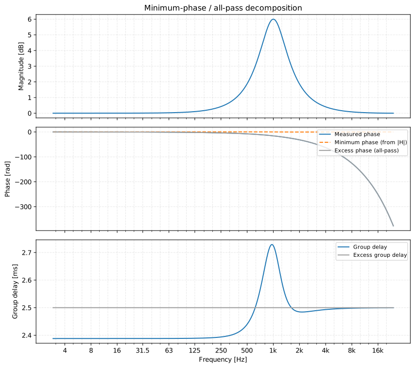

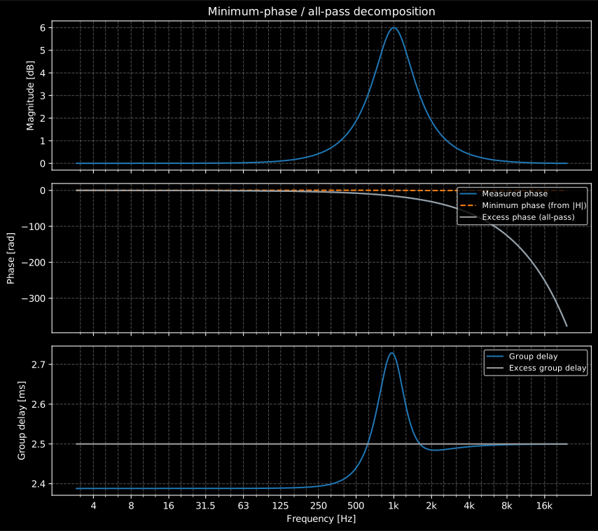
A +6 dB peaking equalizer measured through a 2.5 ms processing latency: the minimum-phase part carries only the small phase wiggle an equalizer could invert, the excess phase is the pure $-2\pi f{t}_0$ ramp of the delay, and the excess group delay reads the latency directly as a flat 2.5 ms line.

In an acoustic measurement that flat part is not latency, it is distance. The time of flight from loudspeaker to microphone is about 2.9 ms per metre, so a response measured at 1 m carries a 2.9 ms excess group delay that has nothing to do with the electronics, and a reader who reads it as processing latency will try to compensate a delay that does not exist. Remove it first — trim the impulse response to its arrival, or subtract the known distance — because nothing else in the excess phase can be interpreted until it is gone. What remains after the removal is the part that matters: an all-pass residue no equalizer can invert, produced by genuinely non-minimum-phase behaviour such as a strong reflection arriving later than the direct sound, or a crossover whose drivers’ acoustic centres are not aligned. That is the design question phase_decomposition is actually asked in loudspeaker and room correction: a response that is minimum phase once the delay is removed can be corrected in magnitude and phase together by a single filter; one that is not, cannot.

Show the code for this figure

import matplotlib.pyplot as plt
import numpy as np
from scipy import signal as sp_signal
from phonometry import phase_decomposition

fs = 48000.0
delay = int(0.0025 * fs)                      # a 2.5 ms processing latency
gain_a = 10.0 ** (6.0 / 40.0)                 # +6 dB peaking EQ at 1 kHz, Q = 1
w0 = 2.0 * np.pi * 1000.0 / fs
alpha = np.sin(w0) / 2.0
b = np.array([1 + alpha * gain_a, -2 * np.cos(w0), 1 - alpha * gain_a])
a = np.array([1 + alpha / gain_a, -2 * np.cos(w0), 1 - alpha / gain_a])
imp = np.zeros(16384)
imp[delay] = 1.0
ir = sp_signal.lfilter(b / a[0], a / a[0], imp)

res = phase_decomposition(np.fft.rfft(ir), fs)
res.plot()   # |H|, the three phases and the group delays
plt.show()

The decomposition $H=H_{\text{min}}{H}_{\text{ap}}$ splits what an equalizer can invert ($H_{\text{min}}$, minimum phase, causal and causally invertible) from what it never can ($H_{\text{ap}}$, the all-pass excess: latency plus non-minimum-phase zeros such as reflections). The excess phase is $0$ for a minimum-phase response and exactly $-2\pi f{t}_0$ for a pure latency $t_0$; its group delay reads the latency in seconds.

Numerical contract, pinned by the tests: on a strictly minimum-phase biquad sampled on a dense grid the reconstructed phase matches the true phase to better than $10^{-12}$ rad; the group delay of a first-order allpass matches the closed form $(1-a^2)/(1+2a\cos \omega +a^2)$ to $10^{-5}$ samples; the excess group delay of a delayed biquad returns the delay to $10^{-6}$ samples. The precautions are documented with the API: the response must be sampled uniformly from DC to Nyquist inclusive (the rfft layout) and densely enough that the underlying impulse response fits the implied record; magnitude zeros (band-pass edges, notch bottoms) are floored and are not representable by a minimum-phase system; the oversample factor (trigonometric interpolation of the magnitude before the cepstrum) mitigates the cepstral aliasing that near-circle zeros cause on coarse grids.

Relation to other tools

• impulse_response recovers the linear IR from the same sweep recording and simply discards the negative-time distortion products; swept_sine_distortion is the tool that reads them.
• thd / harmonic_analysis measure distortion from a steady tone at one frequency; the sweep separator returns the same ratios as a continuous function of frequency, from one measurement. Speed is the least of the reasons to prefer it. Deconvolving a sweep of duration $T$ concentrates the whole excitation into one impulse, so the signal-to-noise ratio of the result exceeds that of the raw recording by roughly $10{\log }_{10}$ of the time-bandwidth product, which is how a sweep measures a quiet device in a room a stepped tone could not work in. And the separation is in time, not in frequency: no notch filter is applied and no bin has to be declared a harmonic, which is what keeps THD(f) meaningful where a device’s own harmonics fall outside its passband. The counterpart is that a reverberant tail outlasting the spacing $L\ln (N/(N-1))$ contaminates the neighbouring order, which is what the sizing rules of section 4 exist to prevent.
• The phase utilities operate on any one-sided complex response: an rfft of a measured IR, or the response of a transfer_function estimate on a uniform grid. minimum_phase alone also accepts a plain magnitude array, e.g. a design target for equalization.

What this guide covers

• Covered

  Farina’s exponential-sweep deconvolution (AES preprint 5093, 2000) and the phase-coherent synchronized swept-sine of Novak, Lotton & Simon (2015): the harmonic separation, the closed-form inverse-filter spectrum and the fractional-sample de-skewing, implemented by swept_sine_distortion and synchronized_sweep_signal. The acquisition conditions the result depends on: the drive level and its amplitude reference, the fade that must reach both calls, the clipping and tail requirements, the time-variance and impulsive-noise failure modes, and the sizing rules that relate $T$, $N$ and $f_2$. The phase utilities minimum_phase, group_delay, excess_phase and phase_decomposition implement the Hilbert-transform relation of Bendat & Piersol Section 13.1.4 through the real cepstrum.

• Not covered

  Intermodulation and dynamic intermodulation distortion (IEC 60268-3, clauses 14.12.7-10) are measured from steady tones on the electroacoustics page, not from a sweep; this page separates harmonic orders only. Müller & Massarani’s sweep monograph is cited for background practice (fades, inverse-filter technique), not for a specific implemented formula. With method="farina", the harmonic phases of $H_2\dots H_N$ are returned but should be ignored: the plain exponential sweep breaks the time-shift/harmonic equivalence the synchronized method relies on. Nothing here checks the acquisition conditions of section 1.1 either: the functions take the arrays they are given, so the drive level, the absence of clipping and the length of the tail are the operator’s to keep and to report.

See also

• Electroacoustics: the steady-tone $\mathrm{THD}$, THD+N and intermodulation set of IEC 60268-3 that this sweep complements, and the operating point they are all defined at.
• Loudspeaker Characterisation (IEC 60268-5): the THD(f) curve produced here is the distortion panel of that rated-characteristics report.
• Room acoustics: impulse_response, which is the linear half of the same recording.
• API reference: electroacoustics.swept_sine and signals.phase.

References

• Bendat, J. S., & Piersol, A. G. (2010). Random data: Analysis and measurement procedures (4th ed.). Wiley. https://doi.org/10.1002/9781118032428Section 13.1.4: the Hilbert-transform relation between log-magnitude and phase behind the minimum-phase reconstruction. ISBN 978-0-470-24877-5.
• Farina, A. (2000). Simultaneous measurement of impulse response and distortion with a swept-sine technique (108th AES Convention, Paris, preprint 5093). The exponential-sweep deconvolution and the L·ln(n) packing of each distortion order ahead of the linear impulse response.
• Müller, S., & Massarani, P. (2001). Transfer-function measurement with sweeps. Journal of the Audio Engineering Society, 49(6), 443-471. The sweep-measurement monograph behind the practice notes: inverse filters, fades and the rejection of distortion from the linear impulse response.
• Novak, A., Lotton, P., & Simon, L. (2015). Synchronized swept-sine: Theory, application and implementation. Journal of the Audio Engineering Society, 63(10), 786-798. https://doi.org/10.17743/jaes.2015.0071The synchronization condition that makes harmonic phases system properties, the closed-form inverse-filter spectrum used for the deconvolution and the fractional-sample separation.