The pressure routes to the sound power level fail exactly where machines live: on a factory floor where the neighbouring lines cannot be switched off. Sound intensity is the net energy flux, so it distinguishes energy leaving the source from steady energy merely passing through the measurement surface, and the scanning methods built on it tolerate extraneous noise that would defeat any pressure method. This guide covers the two of them: the ISO 9614-2 engineering/survey determination with its field indicators and per-band achieved grade, the ISO 9614-3 precision (grade 1) scan with its tighter criteria, and the accredited-style test fiche. The probe itself, its finite-difference bias and the ISO 9614-1 discrete-point method live in Sound Intensity (p-p); which route fits which job is weighed in Sound Power.
1. Intensity scanning (ISO 9614-2)
Section titled “1. Intensity scanning (ISO 9614-2)”A p-p probe (see the Sound Intensity guide) is swept continuously over each of segments of a surface enclosing the source, reporting the segment-averaged signed normal intensity : one row per segment, one column per band.
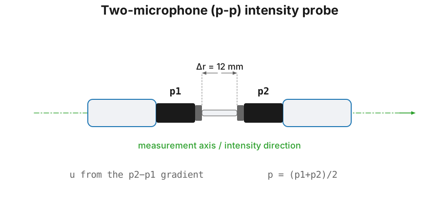
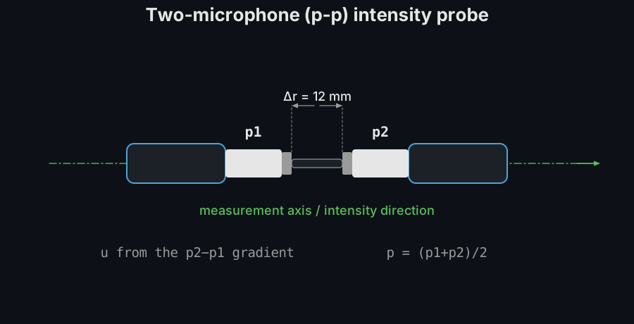
The partial powers sum to the total:
A p-p probe traces the serpentine scan over the top face of the measurement box while the normal-intensity arrows appear behind it, and the partial powers of the five faces accumulate into the sound power level L_W.
A p-p probe traces the serpentine scan over the top face of the measurement box while the normal-intensity arrows appear behind it, and the partial powers of the five faces accumulate into the sound power level L_W.
Running the scan
Section titled “Running the scan”Everything above arrives as an array; this is where it comes from. The measurement surface is divided into at least four segments (clause 8.2), chosen where possible so that a region of net inflow is not averaged together with a region of net outflow, and so that each segment faces one component of the machine. Its mean distance from the source surface is at least 200 mm for an extended vibrating surface, reducible to 100 mm for a small compact source. At that point, action a) of Table B.1 (“move the surface out”) is no longer available to you.
The scan itself is a path, not a set of points. Its basic element is a straight line; the path must cover the segment uniformly at uniform speed, with adjacent lines equally spaced, and on the initial measurement surface the mean line spacing shall not exceed the mean distance from the segment to the source (clause 8.1). Sweep speed is 0,1 m/s to 0,5 m/s by hand, 0 m/s to 1 m/s mechanically; each segment takes at least 20 s, with the time-averaging started and stopped at the segment boundaries so that the reported belongs to that segment and nothing else. The probe axis stays normal to the surface throughout, and the operator stands to the side of the segment being scanned, not in front of it.
For the engineering grade each segment is scanned twice, and the two paths
must be orthogonal: the second sweep rotated 90° wherever that is possible
(clause 8.3.1). That is what normal_intensity_2 is: not a repeat of the same
sweep, but the rotated one. Criterion 3 exists precisely to catch a field that
does not repeat, and repeating an identical path passes it on a determination
that a rotated path would fail. Note 10 of the same clause adds the practical
consequence: above , scan speeds over 0,25 m/s are
likely to fail criterion 3 whatever the stability of the field.
The field indicators and their criteria
Section titled “The field indicators and their criteria”A band whose net power is non-positive (: more energy entering the
surface than leaving it, from a stronger source outside) is not determinable
and reported as NaN (clause 9.2). Two normative field indicators qualify the
bands that are. The surface pressure-intensity indicator measures
how reactive or how contaminated the field is, and the
negative-partial-power indicator measures how much energy
circulates in and out across the surface:
where is the area-weighted surface pressure level over the segments. These are the ISO 9614-2 names for the two ISO 9614-1 Annex A indicators the intensity guide calls and : and for equal-area segments, so the field indicators there and the qualification criteria here are the same two numbers under two standards’ notations.
The probe’s dynamic capability (pressure-residual
intensity index minus the bias factor , 10 dB for grade 2 and 7 dB for
grade 3) must exceed (criterion 1); is
criterion 2 (mandatory for grade 2); and the two rotated sweeps must agree
within the Table 2 limit per segment (criterion 3). A band is
engineering grade
when criteria 1, 2 and 3 hold, survey when 1 and 3 hold, else none.
Reading the indicators
Section titled “Reading the indicators”Neither indicator is a boolean, and both carry a scale. sits near zero when everything the surface encloses radiates outward and nothing else reaches it; a few decibels is normal in-situ work; and clause 8.3.2 asks that every effort be made to keep it below 10 dB by the choice of surface. A large has two causes with opposite fixes: a reactive near field, answered by moving the surface out, and a strong external source, answered by moving the surface in towards the machine or by shielding it. reads differently: zero when every segment radiates outward, and 3 dB when the inward and outward partial powers are already comparable to the net, so above 3 dB the surface is straddling two sources and the fix is to re-cut it. Averaging longer does not help, because the problem is where the surface is, not how noisy the estimate is.
When criterion 1 fails, the remedies are cheap before they are expensive: enlarge the surface away from the near field, shield or remove the extraneous source, fit a larger spacer to raise (see Choosing the probe), and only then consider better hardware. Dropping the claim from engineering to survey grade buys 3 dB of on its own, because goes from 10 dB to 7 dB: the trade-off is the loss of grade.
import numpy as npfrom phonometry import emission
# 6 surface segments x 6 octave bands: signed normal intensity (W/m^2) from two# repeated sweeps, the segment areas, and the per-segment surface SPL (dB).freqs = np.array([125, 250, 500, 1000, 2000, 4000], dtype=float)areas = np.full(6, 0.5)                                 # 0.5 m^2 per segmentrng = np.random.default_rng(0)scan1 = np.abs(rng.normal(1e-4, 2e-5, size=(6, 6)))     # (segments, bands)scan2 = scan1 * (1.0 + rng.normal(0.0, 0.02, size=(6, 6)))pressure = np.full((6, 6), 80.0)
res = emission.sound_power_intensity(    scan1, areas, normal_intensity_2=scan2, pressure_levels=pressure,    pressure_residual_index=12.0, frequencies=freqs,    band_type="octave", grade="engineering",)print(np.round(res.sound_power_level, 1))               # per-band LWprint(round(res.sound_power_level_a, 1))                # LWA over determinable bandsprint(round(float(res.dynamic_capability_index[0]), 1)) # Ld = 12 - 10 = 2.0 dBprint(round(float(res.surface_pressure_intensity_index[0]), 2))   # FpIprint(list(res.achieved_grade))                         # per-band grade
res.plot()   # LW spectrum; non-positive (undeterminable) bands hatched (needs matplotlib)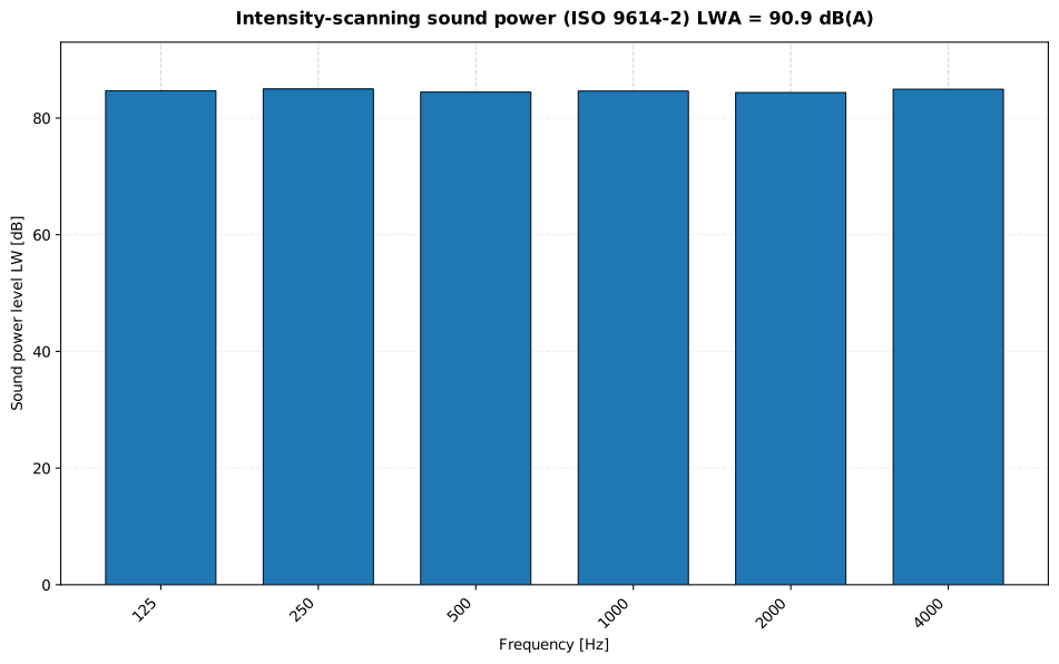
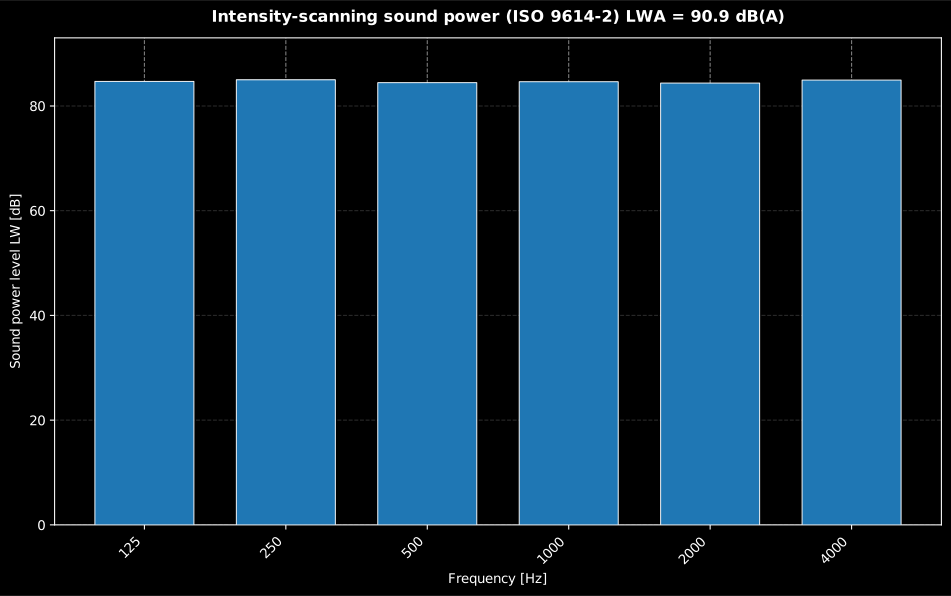
The partial powers of the six segments sum to each band’s ; every band here nets positive power and passes the field-indicator criteria at engineering grade, so all six bars stand, and the A-weighted total of 90.9 dB(A) heads the title.
Show the code for this figure
import matplotlib.pyplot as pltimport numpy as npfrom phonometry import emission
# 6 surface segments x 6 octave bands: signed normal intensity (W/m^2) from two# repeated sweeps, the segment areas, and the per-segment surface SPL (dB).freqs = np.array([125, 250, 500, 1000, 2000, 4000], dtype=float)areas = np.full(6, 0.5)                                 # 0.5 m^2 per segmentrng = np.random.default_rng(0)scan1 = np.abs(rng.normal(1e-4, 2e-5, size=(6, 6)))     # (segments, bands)scan2 = scan1 * (1.0 + rng.normal(0.0, 0.02, size=(6, 6)))pressure = np.full((6, 6), 80.0)res = emission.sound_power_intensity(    scan1, areas, normal_intensity_2=scan2, pressure_levels=pressure,    pressure_residual_index=12.0, frequencies=freqs,    band_type="octave", grade="engineering",)
# res is the SoundPowerIntensityResult computed above. One line:res.plot()plt.show()
# By hand: a bar spectrum of LW with the A-weighted total in the title.freqs = res.frequenciespositions = np.arange(freqs.size)fig, ax = plt.subplots()ax.bar(positions, res.sound_power_level, width=0.7, color="#1f77b4")ax.set_xticks(positions)ax.set_xticklabels([f"{f:g}" for f in freqs], rotation=45, ha="right")ax.set_xlabel("Frequency [Hz]")ax.set_ylabel("Sound power level LW [dB]")ax.set_title(    f"Intensity-scanning sound power (ISO 9614-2)  "    f"LWA = {res.sound_power_level_a:.1f} dB(A)")plt.show()
Supplying normal_intensity_2 (the second, rotated sweep) averages the two for
the
partial powers and evaluates criterion 3; pressure_levels enables ;
pressure_residual_index () plus a second sweep enables the
per-band
achieved grade. The probe’s finite-difference intensity has a
frequency-dependent bias handled in the intensity guide.
Where the A-weighted total loses bands
Section titled “Where the A-weighted total loses bands”sound_power_level_a is not a sum over every band, and the difference matters
for anything that will be compared against a limit. Two things take a band out
of it, for different reasons:
- a band whose net power is non-positive is not determinable at all
(clause 9.2) and comes back
NaN;negative_bandflags it; - a band that is determinable but fails criterion 1, or at engineering grade
criterion 2, is a perfectly good number that clause 10.6 b) forbids you to
include in an A-weighted determination unless its contribution is negligible
per clause 4.3;
a_weighting_omitted_bandsrecords exactly which ones.
Clause 10.6 b) also makes stating that omission part of the determination: an
reported without saying which bands were dropped does not conform. The
consequence is one-directional: the total is an underestimate, and the
reader can bound it by summing the omitted bands at their computed level and
adding them back. Note also the failure mode of the screening itself: without
pressure_levels and pressure_residual_index the criteria cannot be
evaluated, so every determinable band is summed and a SoundPowerWarning says
so. A quiet total is not the same as a screened one.
Criterion 3 is not quite a hard gate
Section titled “Criterion 3 is not quite a hard gate”Criterion 3 is evaluated per segment and per band, which is why repeatability
comes back per segment rather than as one verdict. A failing segment does not
automatically void its band: clause 8.3.1 allows the determination to stand when
the summed partial powers of the failing segments lie more than 10 dB below
the source power obtained from the passing ones, their contribution then being
negligible. What it does not allow is silence: the bands in which criterion 3
was not satisfied must carry a statement in the report that their uncertainty
exceeds the Table 2 value for the intended grade.
The repeatability_limit default deserves the same care. Table 2 tabulates
per band for the engineering grade only; for the survey grade it gives a
single A-weighted value of 4 dB, and this implementation reuses that 4 dB as a
per-band survey limit. That is a deliberate extrapolation, not a normative
value, and it is looser than any grade-2 limit in the table: a survey-grade
criterion-3 pass is therefore not evidence of grade-2 repeatability. Table 2
is also bounded: _table2_s raises outside the octave bands 63 Hz to 4 kHz and
the one-third-octave bands 50 Hz to 6,3 kHz, so an 8 kHz octave is an
exception, not a wide limit.
The instrument and the environment
Section titled “The instrument and the environment”The fiche’s "Class 1 p-p intensity probe (IEC 61043)" is a claim with clauses
behind it. The instrument including its probe shall comply with IEC 61043,
verified in a laboratory at least annually, or at least every two years if an
intensity calibrator is applied before each power determination (clause 6.2).
Before each series, a class 0 or class 1 IEC 60942 calibrator goes on each probe
microphone (clause 6.2.1), and the probe-reversal test of clause 6.2.2 confirms
in situ that the chain agrees on which way is out; both procedures, and what
their failures mean, are in
Sound Intensity.
Clause 10.5 makes reporting both of them part of the deliverable.
The environment has limits too. The mean air-flow velocity over the measurement surface shall be below 4 m/s, or a windscreen shall be used (clause 6.1); static pressure and temperature are measured because they set the density and the speed of sound the intensity is computed with.
When a criterion fails, Annex B’s Table B.1 lists what to change rather than
leaving it at a False: increase the averaging or the scan time, move the
measurement surface, double the scan-line density, subdivide the surface into
more segments, or shield the extraneous source. The action codes are keyed to
which criterion failed, which is why the result reports the criteria separately
instead of one boolean.
sound_power_intensity() parameters
Section titled “sound_power_intensity() parameters”| Parameter | Type | Units | Range / default | Notes |
|---|---|---|---|---|
normal_intensity | 2D array | W/m² | (N_seg, N_bands) | Signed segment-averaged normal intensity (first sweep) |
areas | 1D array | m² | > 0, (N_seg,) | Segment areas |
normal_intensity_2 | 2D array | W/m² | same shape | Second sweep → criterion 3 and averaging |
pressure_levels | 2D array | dB | same shape | Segment SPL → |
pressure_residual_index | float or 1D array | dB | — | → / criterion 1 |
frequencies | 1D array | Hz | octave 63 Hz-4 kHz, third 50 Hz-6,3 kHz | and Table 2 limits; outside the range Table 2 has no and the call raises |
band_type | str | — | 'third' (default) / 'octave' | Table 2 lookup |
grade | str | — | 'engineering' (default) / 'survey' | Selects |
repeatability_limit | float or 1D array | dB | default Table 2 (survey: the A-weighted 4 dB reused per band) | Override criterion-3 |
Returns a SoundPowerIntensityResult: partial_power/partial_power_level
per segment and band, sound_power/sound_power_level (band total, NaN
where negative_band), negative_band (the non-determinable bands),
surface_pressure_intensity_index (),
negative_partial_power_index (), repeatability,
dynamic_capability_index (), achieved_grade,
a_weighting_omitted_bands (the bands clause 10.6 b) kept out of ),
surface_area, sound_power_level_a and grade.
partial_power_level is the field that pays for the whole method. A pressure
determination returns one number per band; an intensity scan returns one per
segment and band, signed, so the result says where the power leaves the
machine and where it flows back in:
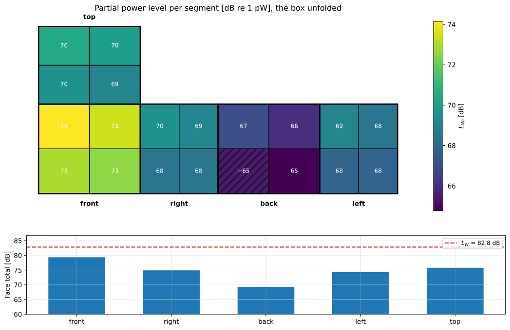
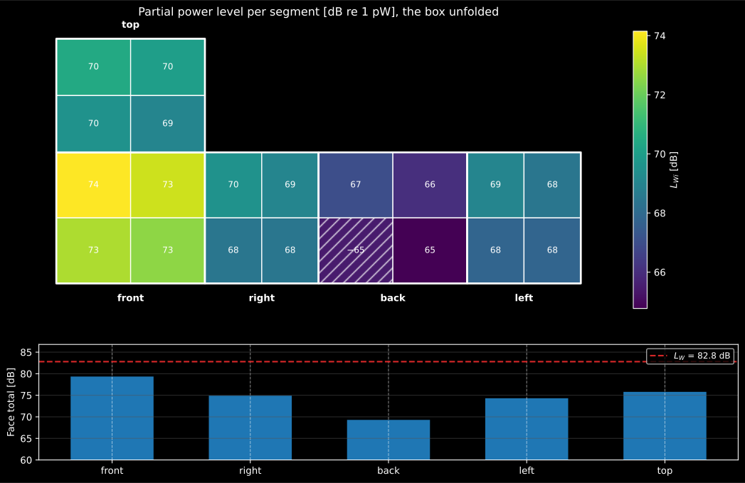
The measurement box unfolded, one tile per segment. The front face carries most of the emission; the hatched segment on the shadow side nets inward, which is normal beside a louder neighbour and is exactly what counts. A band-summed spectrum cannot show any of this, and it is the map, not the spectrum, that tells you which panel to treat.
Show the code for this figure
import matplotlib.patches as mpatchesimport matplotlib.pyplot as pltimport numpy as np
# A 1.2 x 0.8 x 1.0 m machine boxed at d = 0.25 m: five faces, four segments# each, one of them taking net inflow from a louder neighbour.face_area = np.array([1.7 * 1.5, 1.3 * 1.5, 1.7 * 1.5, 1.3 * 1.5, 1.7 * 1.3])seg_area = np.repeat(face_area / 4.0, 4)share = np.array([2.6, 2.2, 2.0, 1.8, 0.9, 0.8, 0.7, 0.7,                  0.5, 0.4, -0.35, 0.3, 0.8, 0.7, 0.6, 0.6,                  1.1, 1.0, 0.9, 0.8])res = emission.sound_power_intensity(    (share * 1.0e-5 / seg_area)[:, None], seg_area,    frequencies=np.array([500.0]))level, signed = res.partial_power_level[:, 0], res.partial_power[:, 0]
# The developed net: four side faces in a row, the top above the front.origin = ((0, 0), (1.7, 0), (3.0, 0), (4.7, 0), (0, 1.5))size = ((1.7, 1.5), (1.3, 1.5), (1.7, 1.5), (1.3, 1.5), (1.7, 1.3))fig, ax = plt.subplots(figsize=(11, 5))for f, ((ox, oy), (w, h)) in enumerate(zip(origin, size, strict=True)):    for k in range(4):        value = level[4 * f + k]        ax.add_patch(mpatches.Rectangle(            (ox + (k % 2) * w / 2, oy + (1 - k // 2) * h / 2), w / 2, h / 2,            facecolor=plt.get_cmap("viridis")(                (value - level.min()) / (level.max() - level.min())),            edgecolor="black",            hatch="//" if signed[4 * f + k] < 0 else None))ax.set(xlim=(-0.2, 6.2), ylim=(-0.4, 3.0), aspect="equal")plt.show()
2. Precision intensity scanning (ISO 9614-3)
Section titled “2. Precision intensity scanning (ISO 9614-3)”ISO 9614-3 is the grade-1 scanning method: like ISO 9614-2 it integrates the normal intensity over a surface enclosing the source, but with a continuous scan, tighter field-indicator criteria and an explicit uncertainty budget.
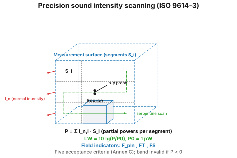
Power and level (Clause 7). The partial power of each segment is ; the total gives , . A band whose net power is non-positive () is flagged not-applicable rather than logged. The field indicators (temporal variability , the signed and unsigned pressure–intensity indicators, and the non-uniformity ) drive the five acceptance criteria.
import numpy as npfrom phonometry import emission
# A fully enclosing surface with a uniform normal intensity In = W/S recovers# the source power exactly: LW = 10*lg(W/P0). Here W = 100 uW -> 80 dB.areas = np.array([0.5, 1.0, 0.25, 2.0])w = 1.0e-4i_n = np.full(areas.shape, w / float(areas.sum()))res = emission.sound_power_intensity_precision(i_n, areas)print(round(float(res.sound_power[0]), 6))          # 0.0001print(round(float(res.sound_power_level[0]), 2))    # 80.0
Across several bands the result carries the per-band (NaN where the net
power is non-positive), flags those bands not_applicable, and draws them
with the one-line result.plot() of the figure below:
import numpy as npfrom phonometry import emission
# Four partial surfaces scanned over five one-third-octave bands. Each cell of# partial_intensity is the signed normal intensity In_i (W/m^2); areas are the# partial-surface areas Si. The 250 Hz band has net-negative power (a locally# reactive field), so ISO 9614-3 flags it not-applicable (clause 9.2) -> NaN.freqs = np.array([250, 500, 1000, 2000, 4000], float)areas = np.array([0.5, 1.0, 0.75, 0.5])base_intensity = np.array([2.0e-6, 8.0e-6, 2.0e-5, 1.0e-5, 3.0e-6])partial_intensity = base_intensity[None, :] * np.array([1.0, 1.1, 0.9, 1.05])[:, None]partial_intensity[:, 0] = [2.0e-6, -3.0e-6, -4.0e-6, -1.0e-6]   # net-negative band
result = emission.sound_power_intensity_precision(partial_intensity, areas, frequencies=freqs)print(result.not_applicable_band.tolist())   # [True, False, False, False, False]print(round(result.sound_power_level_a, 1))   # 80.6result.plot()   # LW spectrum; the not-applicable band is hatched (needs matplotlib)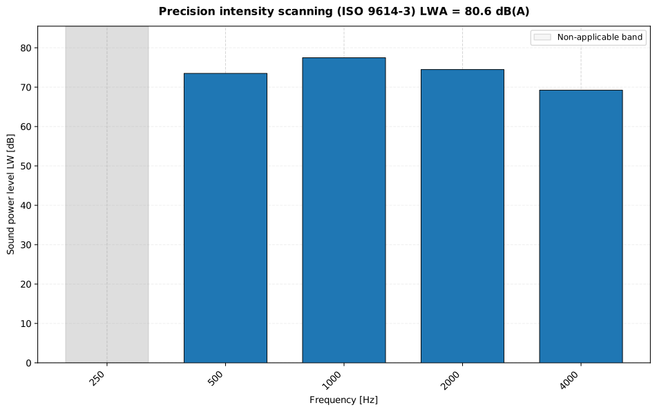
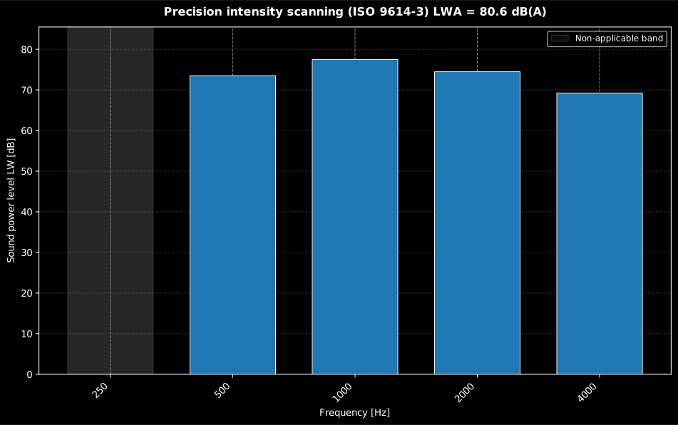
The 250 Hz band nets negative (more energy flowing in than out), so ISO 9614-3 declares it not-applicable; the figure hatches and greys it while the four determinate bands and the A-weighted total stand.
Show the code for this figure
import matplotlib.pyplot as pltimport numpy as npfrom phonometry import emission
# Four partial surfaces scanned over five one-third-octave bands. Each cell of# partial_intensity is the signed normal intensity In_i (W/m^2); areas are the# partial-surface areas Si. The 250 Hz band has net-negative power (a locally# reactive field), so ISO 9614-3 flags it not-applicable (clause 9.2) -> NaN.freqs = np.array([250, 500, 1000, 2000, 4000], float)areas = np.array([0.5, 1.0, 0.75, 0.5])base_intensity = np.array([2.0e-6, 8.0e-6, 2.0e-5, 1.0e-5, 3.0e-6])partial_intensity = base_intensity[None, :] * np.array([1.0, 1.1, 0.9, 1.05])[:, None]partial_intensity[:, 0] = [2.0e-6, -3.0e-6, -4.0e-6, -1.0e-6]   # net-negative bandresult = emission.sound_power_intensity_precision(partial_intensity, areas, frequencies=freqs)
# result is the PrecisionIntensityResult computed above. One line:result.plot()plt.show()
# By hand: determinate bands as LW bars; a not-applicable band (its LW is NaN)# is flagged by a full-height greyed, hatched span rather than a zero-height bar.freqs = result.frequenciespositions = np.arange(freqs.size)neg = result.not_applicable_bandlw = np.nan_to_num(result.sound_power_level)fig, ax = plt.subplots()ax.bar(positions[~neg], lw[~neg], width=0.7, color="#1f77b4")for pos in positions[neg]:    ax.axvspan(pos - 0.35, pos + 0.35, facecolor="#888888", alpha=0.28,               hatch="//", edgecolor="#888888")ax.set_xticks(positions)ax.set_xticklabels([f"{f:g}" for f in freqs], rotation=45, ha="right")ax.set_xlabel("Frequency [Hz]")ax.set_ylabel("Sound power level LW [dB]")ax.set_title(    f"Precision intensity scanning (ISO 9614-3)  "    f"LWA = {result.sound_power_level_a:.1f} dB(A)")plt.show()
Qualifying the scan (Annex C)
Section titled “Qualifying the scan (Annex C)”sound_power_intensity_precision returns a power, not a grade: nothing in that
result says whether the determination is a grade-1 one. The acceptance gate is a
separate pair of calls, and without it the precision half of this page is a
computation with its criteria removed.
precision_field_indicators computes the Annex B indicators from the same
segment arrays: the signed and unsigned pressure-intensity indicators
, the field non-uniformity , and the temporal variability
when a per-time-window intensity is supplied. precision_qualification then
evaluates the five Annex C criteria per band:
- scan repeatability, with from Table 1 (Eq. C.1): half the tolerance ISO 9614-2 allows, which is most of what “precision” costs;
- dynamic-capability adequacy, with and dB (Eq. C.2);
- dB (Eq. C.3), the precision counterpart of ISO 9614-2’s limit;
- field non-uniformity, (Eq. C.4);
- scan-density convergence, between the initial density and a doubled one (Eq. C.5).
The conjunction is qualified, and it carries one subtlety worth knowing before
you re-scan a machine: clause C.1.6.2 accepts a band that satisfies criterion 5
as a final result even where criterion 4 is not met. A non-uniform field
that stops changing when the scan density doubles has been sampled adequately;
it is the change with density, not the non-uniformity itself, that invalidates.
# The same four segments and five bands, now with their surface pressure levels# and a second (90-degree rotated, doubled-density) scan: enough for Annex C.segment_pressure = np.full((4, 5), 74.0)ind = emission.precision_field_indicators(partial_intensity, segment_pressure)print(np.round(ind.f_pi_signed, 1))            # [12.2  4.9  0.9  3.9  9.2]
scan1 = 10.0 * np.log10(np.abs(partial_intensity.mean(axis=0)) / 1e-12)scan2 = scan1 + np.array([0.9, 0.2, 0.1, 0.3, 0.4])crit = emission.precision_qualification(    ind, scan_intensity_level_1=scan1, scan_intensity_level_2=scan2,    pressure_residual_index=15.0,              # Ld = 15 - 10 = 5 dB    field_nonuniformity_1=ind.fs, field_nonuniformity_2=0.95 * ind.fs,    frequencies=freqs,)print(crit.criterion_2.tolist())   # [False, True, True, True, False]print(crit.qualified.tolist())     # [False, True, True, True, False]
Two bands fail here, and they fail for the reason the numbers say: at 250 Hz and at 4 kHz the signed indicator (12.2 dB and 9.2 dB) exceeds the probe’s dB, so the instrument cannot resolve the net flux against its own residual index. That is criterion 2, and the answer is a better probe, a larger spacer or a surface moved away from the reactive near field. A longer scan will not help.
3. The measurement report (.report())
Section titled “3. The measurement report (.report())”The intensity-scanning result (SoundPowerIntensityResult, ISO 9614-2) writes
a one-page PDF fiche laid out like a sound-power test sheet through its own
.report(), sharing the layout and the ReportMetadata container of the
pressure-method fiche.
The standard-basis line
names ISO 9614-2:1996 and the measurement grade, the per-band table lists the
intensity-derived band sound-power level , and the boxed carries
the total , the measurement surface and the determination grade
(the intensity result has no expanded uncertainty ). verbose=True adds the
field indicators (surface pressure-intensity) and
(negative partial power) and the per-band achieved grade; the basis strip
states the partial-power model (the segment partial powers
summing to ) and the Annex B qualification criteria. A band whose net power
is non-positive is not determinable (clause 9.2) and prints an em dash.
import numpy as npfrom phonometry import ReportMetadata, emission
freqs = np.array([125, 250, 500, 1000, 2000, 4000], float)# Six equal 0.5 m^2 segments (S = 3.0 m^2); one uniform normal-intensity# spectrum scanned twice, with the surface SPL and the instrument residual# index that qualify every band at engineering grade.intensity = np.array([0.6e-4, 1.0e-4, 1.5e-4, 1.4e-4, 0.9e-4, 0.5e-4])scan = np.tile(intensity, (6, 1))res = emission.sound_power_intensity(    scan, np.full(6, 0.5), normal_intensity_2=scan.copy(),    pressure_levels=np.full((6, 6), 80.0), pressure_residual_index=15.0,    frequencies=freqs, band_type="octave", grade="engineering",)
res.report(    "sound_power_intensity.pdf",    metadata=ReportMetadata(        client="Example manufacturing plant",        specimen="Hydraulic power pack (floor-standing)",        test_room="Machine hall with steady background noise",        instrumentation="Class 1 p-p intensity probe (IEC 61043), s/n 0042",        laboratory="Phonometry reference example",        report_id="EXAMPLE-9614",        requirement=93.0,    ),)   # LWA = 90.9 dB(A) re 1 pW -> declared limit 93 dB(A): PASS
The example fiche is regenerated with make reports and kept rendered in the
repository; click the preview to open the PDF.
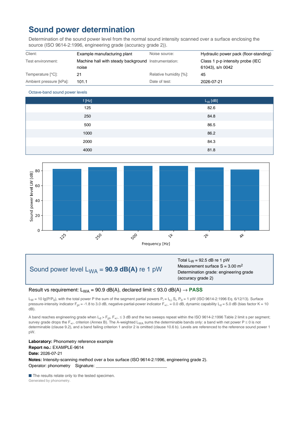
One-page ISO 9614-2 sound-power-by-intensity determination fiche: a header with the client, the noise source, the machine-hall test environment and the intensity probe and climate, the octave-band table (125 Hz to 4 kHz) of intensity-derived band sound-power levels LW, the sound-power spectrum LW(f) with a nominal band axis, the boxed A-weighted sound power level LWA = 90.9 dB(A) re 1 pW with the total LW = 92.5 dB, the measurement surface S = 3.00 m2 and the engineering grade, and a PASS verdict against the declared 93 dB(A) limit, closed by a basis strip stating the partial-power model, the field indicators FpI and F+/- and the Annex B qualification criteria.
The precision sheet (ISO 9614-3)
Section titled “The precision sheet (ISO 9614-3)”PrecisionIntensityResult writes its own fiche, and it is not the part 2 sheet
with a different title: part 3 asks a report to state different things
(clause 10). The per-band table carries the normalized level the
standard reports (Eq. 10) beside , and the expanded uncertainty of
clause 4.3, twice the Table 1 standard deviation of reproducibility of the
band; the caption names the frequency range the determination covers, because
clause 4.3 asks for it whenever that range is narrower than 50 Hz to 6.3 kHz. A
one-third-octave set is printed in two column groups side by side, the way an
accredited sheet fits that many bands on a page. verbose=True tabulates the
four Annex B indicators , , and per band, the
tabulation clause 10 f) 1) asks for, over the measurement surface as Annex B
defines them, and the qualification cell the criteria decide.
Hand it an Annex C qualification and the sheet does what
clause 10 f) 2) makes mandatory: the bands whose Annex C criteria are not
satisfied are dropped from the A-weighted determination and named on the sheet,
next to the bands the method is not applicable to at all (clause 9.2). That is
why the boxed can differ from result.sound_power_level_a, which is
computed before any criterion is evaluated and therefore sums every applicable
band. Beside it the box states the normalized , since clause 10 f) 2)
reports the normalized quantity while the headline number is the level a
declared limit is written against. Without criteria the fiche boxes the result’s own value and says that
no qualification was supplied. residual_index puts the probe’s
pressure-residual intensity index on the sheet (clause 10 d) 5)) with the
dynamic capability it yields; the clause 10 items that are free
description rather than numbers, the scan geometry and speed, the scanning
time and the probe-reversal checks, go in the metadata notes.
import numpy as npfrom phonometry import ReportMetadata, emission
# A box measurement surface: five partial surfaces, each scanned in four# segments, over the one-third-octave bands 200 Hz to 800 Hz. Part 3 works in# one-third octaves, which is the band set Table 1 tabulates its uncertainty# and its criterion-1 tolerance for.third_octave = np.array([200, 250, 315, 400, 500, 630, 800], float)faces = np.array([1.65, 1.575, 1.575, 1.155, 1.155])scanned = 1.2e-5 * np.array([1.3, 1.1, 0.8, 0.9, 0.9])[:, None] * np.ones(7)segment_intensity = np.repeat(scanned, 4, axis=0)# The pressure-intensity margin per band: 8 dB at 200 Hz, where the hall is# reverberant, 2 dB above it.margin = np.array([8.0, 2.0, 2.0, 2.0, 2.0, 2.0, 2.0])segment_levels = 10 * np.log10(segment_intensity / 1e-12) + margin
precise = emission.sound_power_intensity_precision(    scanned, faces, frequencies=third_octave,    temperature_c=28.0, barometric_pressure_pa=94_000.0,)annex_b = emission.precision_field_indicators(segment_intensity, segment_levels)scan_intensity = np.average(scanned, axis=0, weights=faces)  # unequal facesscan_level = 10 * np.log10(scan_intensity / 1e-12)annex_c = emission.precision_qualification(    annex_b, scan_intensity_level_1=scan_level,    scan_intensity_level_2=scan_level + 0.1,    pressure_residual_index=15.0,          # Ld = 15 - 10 = 5 dB    frequencies=third_octave,)print(annex_c.qualified.tolist())   # [False, True, True, True, True, True, True]
precise.report(    "sound_power_intensity_precision.pdf",    metadata=ReportMetadata(        client="Example manufacturing plant",        specimen="Hydraulic power pack (floor-standing)",        test_room="Machine hall with steady background noise",        instrumentation="Class 1 p-p intensity probe (IEC 61043), 12 mm spacer",        temperature_c=28.0, relative_humidity_percent=40.0, static_pressure_kpa=94.0,        laboratory="Phonometry reference example",        report_id="EXAMPLE-9614-3",        requirement=98.0,        notes="Box surface at 0,25 m; five partial surfaces scanned twice.",    ),    indicators=annex_b, criteria=annex_c, residual_index=15.0,)   # 200 Hz fails criterion 2 and is named as omitted from LWA
The example fiche in the repository is a fuller determination of the same machine: sixteen one-third-octave bands from 100 Hz to 3150 Hz over a five-face box surface, with the 100 Hz band failing criterion 2 and named as omitted.
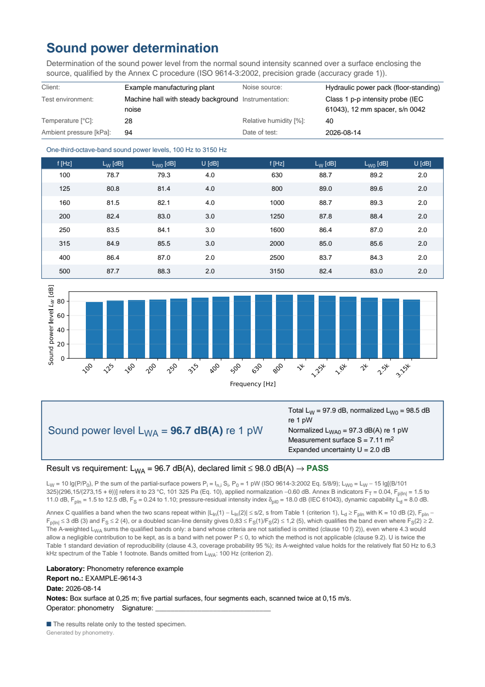
One-page ISO 9614-3 precision sound-power-by-intensity determination fiche: a header with the client, the noise source, the machine-hall test environment, the intensity probe and the 28 degrees Celsius and 94 kPa test atmosphere, the one-third-octave table from 100 Hz to 3150 Hz in two column groups giving the band sound-power level LW, the normalized level LW0 and the expanded uncertainty U, the sound-power spectrum LW(f) with a nominal band axis, the boxed A-weighted sound power level LWA = 96.7 dB(A) re 1 pW with the total LW = 97.9 dB, the normalized total LW0 = 98.5 dB, the normalized A-weighted level LWA0 = 97.3 dB(A), the measurement surface S = 7.11 m2 and the expanded uncertainty U = 2.0 dB, and a PASS verdict against the declared 98 dB(A) limit, closed by a basis strip stating the partial-power model, the meteorological normalization, the Annex B field indicators and the five Annex C criteria, and naming the 100 Hz band as omitted from LWA for criterion 2.
What this guide covers
Section titled “What this guide covers”Covered
The ISO 9614-2 scanning determination (
sound_power_intensity): the partial powers, the surface pressure-intensity and negative-partial-power field indicators, the dynamic capability , the repeatability criterion, the per-band achieved grade and the clause 9.2 not-applicable flagging for net-inflow bands, with the clause 10.6 b) screening of the A-weighted total (a_weighting_omitted_bands). The ISO 9614-3 precision determination (sound_power_intensity_precision) with its own not-applicable flagging, its Annex B field indicators (precision_field_indicators) and the five Annex C acceptance criteria (precision_qualification). Both results render the accredited-style sound-power fiche through.report(), each stating what its own part asks a report to state: the precision sheet adds the normalized levels , the per-band expanded uncertainty of Table 1, the Annex B indicator tabulation and the clause 10 f) 2) omission of the bands the Annex C criteria reject.Not covered
ISO 9614-1, the discrete fixed-point intensity method, is not one of the routes here: it holds the probe still at each position instead of sweeping it, and both its power determination and the Annex A field indicators the two scanning parts reuse are in the sound intensity guide. The probe’s finite-difference bias and the pressure-residual intensity index are measured properties of the instrument, covered in the same guide. Choosing among the seven routes, and the ISO 4871 declaration a result feeds, live in Sound Power.
References
Section titled “References”- Fahy, F. J. (1995). Sound intensity (2nd ed.). E&FN Spon. https://doi.org/10.4324/9780203475386ISBN 978-0-419-19810-9. The monograph on sound energy flux: why intensity separates the energy leaving the source from steady energy passing through, behind both scanning methods.
- International Organization for Standardization. (1996). Acoustics — Determination of sound power levels of noise sources using sound intensity — Part 2: Measurement by scanning (ISO 9614-2:1996). The scanning method of section 1: the partial powers, the FpI and F+/- field indicators and the grade criteria.
- International Organization for Standardization. (2002). Acoustics — Determination of sound power levels of noise sources using sound intensity — Part 3: Precision method for measurement by scanning (ISO 9614-3:2002). The grade-1 scanning method of section 2, its field indicators and the clause 9.2 not-applicable flagging.