Duct-Borne Noise: Fan to Room

Air-conditioning noise is not predicted, it is accounted for. You start from the sound power the fan puts into the duct, walk down the path, and at every element subtract what it attenuates and add back what its own airflow regenerates. What survives to the terminal device is turned into a sound pressure level by the room, the supply and the return paths are added together, and the total is laid against the design criterion. If it fails, the sheet itself tells you which element to change: the row with the small attenuation, or the row whose self-noise is now the floor.

That bookkeeping is what noise_control.duct_path implements, with the element models of noise_control.hvac feeding it and noise_control.duct_modes marking the frequency above which the whole one-dimensional picture stops being exact. The reference throughout is Long, Architectural Acoustics (2nd ed.), Chapters 13 and 14, whose Table 14.9 is the worked sheet this guide is built around, with the ASHRAE HVAC Applications Handbook Chapter 49 for the air terminal devices and Bies, Hansen & Howard for the splitter silencers and the plenums. The reactive four-pole silencers of Silencers and the rest of the installation methods in Industrial noise control are the companion pages.

1. The sheet, and how it adds up

A duct-borne calculation is a table: octave bands across the columns (63 Hz to 8 kHz, the range the published procedures use), one block of rows per physical element. Each block prints what the element takes out, the running level after subtracting it, what the element puts back, and the level leaving it. DuctElement carries exactly the two spectra an element owns, and duct_path walks them:

from phonometry import DuctElement, duct_path

bands = [63.0, 125.0, 250.0, 500.0, 1000.0, 2000.0, 4000.0, 8000.0]
fan = [90.0, 86.0, 82.0, 79.0, 77.0, 75.0, 71.0, 61.0]

path = duct_path(
    bands, fan,
    [
        DuctElement("Elbow, 36 x 24 in, unlined",
                    attenuation=[0, 1, 2, 3, 3, 3, 3, 3],
                    self_noise=[41, 39, 36, 29, 20, 6, 0, 0], code="2"),
        DuctElement("Silencer, 3 ft, standard pressure drop",
                    attenuation=[7, 12, 16, 28, 35, 35, 28, 17],
                    self_noise=[49, 43, 44, 42, 42, 45, 35, 24], code="3"),
    ],
    source_label="Fan, centrifugal FC, 5000 cfm, 2 in w.g.",
)

for row in path.table():
    print(f"{row['code']:>2} {row['label'][:38]:<38} "
          f"{[round(float(v)) for v in row['values']]}")

 S Fan, centrifugal FC, 5000 cfm, 2 in w. [90, 86, 82, 79, 77, 75, 71, 61]
 2 Elbow, 36 x 24 in, unlined             [0, -1, -2, -3, -3, -3, -3, -3]
   Sum                                    [90, 85, 80, 76, 74, 72, 68, 58]
   Self-noise                             [41, 39, 36, 29, 20, 6, 0, 0]
   Combined                               [90, 85, 80, 76, 74, 72, 68, 58]
 3 Silencer, 3 ft, standard pressure drop [-7, -12, -16, -28, -35, -35, -28, -17]
   Sum                                    [83, 73, 64, 48, 39, 37, 40, 41]
   Self-noise                             [49, 43, 44, 42, 42, 45, 35, 24]
   Combined                               [83, 73, 64, 49, 44, 46, 41, 41]
Lp Received level                         [83, 73, 64, 49, 44, 46, 41, 41]

Three conventions matter, and they are worth stating once because every published sheet states them differently. All three can be read off the rows above.

Attenuations are positive. Every element model in noise_control.hvac returns a loss as a positive number of decibels, and the cascade subtracts it. Printed worksheets show the same quantity as a negative level change, so DuctPathResult.table() flips the sign back for the "attenuation" rows: the table reads like the reference, the arithmetic does not have to. The minus signs on the two element rows above are that flip, not a subtraction the reader has to make.

Regenerated noise adds on a power basis. The self-noise of an element is a sound power level in its own right, not a correction to the incoming level, so it is combined as $10{\log }_{10}(10^{L/10}+10^{L_{\text{sn}}/10})$ rather than added arithmetically. That is why the Self-noise row sits between the Sum and the Combined row and never touches the attenuation. Watch the silencer’s triple above: at 63 Hz the running level is 83 dB and the self-noise 49 dB, so the combination is still 83 dB and the silencer’s own noise is invisible; at 2 kHz the attenuation has done its work, the sum is down to 37 dB against a self-noise of 45 dB, and the combination comes out at 46 dB — the element bought to remove the fan is now the loudest thing in that band.

There is a self-noise floor. Long’s sheet uses a 0 dB sound power level wherever an element has no regenerated-noise data, and also as a floor under any computed level that would go negative, which is why his received spectrum bottoms out near 0 dB instead of running off to minus infinity. self_noise_floor reproduces that (default 0.0) and None switches it off entirely; it engages in the 4 kHz and 8 kHz rows of the full sheet in section 6, where the supply path runs past it.

2. The source: fan sound power

The fan is the one element whose spectrum you can build from the operating point alone. fan_sound_power implements the ASHRAE scaling law printed as Long Eq. 13.1,

$$L_W=K_F+10{\log }_{10}\frac{Q_F}{Q_{\text{REF}}}+10{\log }_{10}\frac{P_F}{P_{\text{REF}}}+C_{\text{EFF}}+C_{\text{BFI}},$$

with the spectral constant $K_F$ of Table 13.5 (one row per fan type), the off-peak efficiency correction $C_{\text{EFF}}$ of Table 13.6 and the blade frequency increment $C_{\text{BFI}}$ of Table 13.7 dropped into the single octave band that contains the blade passing frequency. In SI the references are $Q_{\text{REF}}=0.472$ L/s and $P_{\text{REF}}=249$ Pa, so the two logarithmic terms take the same values as the foot-pound form in cfm and inches of water gauge.

from phonometry import (
    blade_passing_frequency, fan_casing_attenuation,
    fan_efficiency_correction, fan_sound_power,
)

CFM, IN_WG = 0.0004719474432, 249.0

fan = fan_sound_power(volume_flow=5000 * CFM, static_pressure=2 * IN_WG,
                      fan_type="forward_curved", relative_efficiency=80.0)
print([round(float(v)) for v in fan.values])
# [99, 99, 89, 84, 82, 77, 72, 67]

print(fan_efficiency_correction(80.0))          # 6.0 dB off the peak
print(blade_passing_frequency(1200.0, 24))      # 480.0 Hz, in the 500 Hz band
print(fan_casing_attenuation().values)          # what the housing holds back
# [ 0.  0.  5. 10. 15. 20. 22. 25.]
fan.plot()                                      # the band spectrum, one line

The fan_type string is the first decision of the whole calculation and the largest single lever in it, because it selects the row of Table 13.5 that sets both the level and the shape. The function takes "airfoil_large" and "airfoil_small" (backward-curved or backward-inclined centrifugal wheels above and below 36 in), "forward_curved", three radial rows by total pressure, three "vaneaxial_hub_*" rows by hub ratio, two "tubeaxial_*" rows by wheel diameter, and "propeller". Ranked as a designer ranks them: the airfoil and backward-inclined centrifugals are the quiet, efficient choice for ducted air (86/86/88/80/76/69/65/63 dB for this duty), forward-curved wheels are cheap and compact but much noisier at low frequency (99/99/89/…), and vaneaxial and propeller fans put their energy into the mid and high bands (propeller: 99/97/104/102/101/98/92/88 dB). The spectrum shape changes with the row, not only the level, so the choice decides which silencer will be needed.

$1200$ in blade_passing_frequency(1200.0, 24) is the shaft speed in revolutions per minute and 24 the blade count; the increment $C_{\text{BFI}}$ it produces is dropped whole into the single octave band containing the result. A fan whose blade tone lands in the band that already governs the design is worth reselecting rather than silencing. And because that increment represents a pure tone inside an octave band, a sheet that passes on band levels can still be judged intrusive — one of the limits listed at the end of this guide.

Two habits keep this honest. The law assumes ideal inlet and outlet flow conditions, so a fan boxed into a plant room with a bad inlet is louder than it says; and ASHRAE’s own current guidance is that a fan’s sound power “is best obtained from manufacturers’ test data” to AMCA Standard 300 or ASHRAE Standard 68. Treat Eq. 13.1 as the early-design fallback, not as the answer. What that test is matters too: ISO 5136 determines the sound power a fan radiates into a duct with an in-duct microphone carrying a slit sampling tube behind a turbulence screen, precisely because a bare microphone in a flowing duct measures its own wind noise long before it measures the fan (the standard puts the ceiling at 15 m/s for a foam ball, 20 m/s for a nose cone and 40 m/s for the sampling tube). So a fan’s duct-borne sound power cannot be obtained by standing beside the machine with a sound level meter: that measures the casing-radiated power of fan_casing_attenuation instead, which is the other row of the same source. The fan radiates the same power from its intake and from its discharge, which is why the supply and return paths of a real sheet start from the same row.

fan_efficiency_correction is a step function, and a brutal one: a fan running at 90 per cent of its peak static efficiency adds nothing, one at 80 per cent adds 6 dB, one below 50 per cent adds 16 dB. Selecting a fan away from its best point is the cheapest way to lose a duct-noise budget before any silencer is priced. fan_casing_attenuation (Table 13.8) is the other side of the same source: the power the housing radiates into the plant room instead of into the duct, zero at 63 and 125 Hz because a vibrating casing radiates low frequency as freely as the unhoused fan.

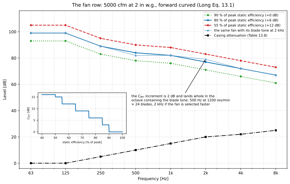
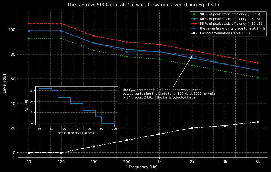
The source row, and the two decisions inside it. The efficiency staircase of the inset is a level shift of the whole spectrum, so a fan selected 25 points off its best point costs 12 dB before any silencer is priced — more than most lined duct runs buy back. The blade increment is small (2 dB for this fan type) but it lands whole in one octave, so what matters is which one. The casing curve is not a loss on this path at all: it is the power the housing radiates into the plant room instead of into the duct.

Show the code for this figure

import matplotlib.pyplot as plt

# `fan_sound_power`, `fan_casing_attenuation` and `fan_efficiency_correction`
# are imported above; CFM and IN_WG are the two unit constants.
duty = dict(volume_flow=5000 * CFM, static_pressure=2 * IN_WG,
            fan_type="forward_curved")

# One line for one fan: the band spectrum.
fan_sound_power(relative_efficiency=80.0, **duty).plot()
plt.show()

fig, ax = plt.subplots()
for efficiency in (90.0, 80.0, 55.0):
    res = fan_sound_power(relative_efficiency=efficiency, **duty)
    ax.semilogx(res.frequencies, res.values, "o-",
                label=f"{efficiency:.0f} % of peak")
casing = fan_casing_attenuation()
ax.semilogx(casing.frequencies, casing.values, "s-.", label="Casing")
ax.set_xlabel("Frequency [Hz]"); ax.set_ylabel("Level [dB]")
ax.legend()
plt.show()

3. What the run takes out

Everything between the fan and the room removes something, and most of it is free. The models are Long Chapter 14 with the Reynolds (1990) regressions, and they all return an HvacSpectrumResult with .values, .plot() and .report(). Every model takes the analysis bands as its first argument, and None means the default hvac.OCTAVE_BANDS, the 63 Hz to 8 kHz set the published sheets use; pass your own vector when the sheet runs on different bands.

Straight ducts. An unlined rectangular duct loses energy into the induced motion of its own walls, so the loss grows with the perimeter-to-area ratio: a wide shallow duct has floppier side walls than a square one. unlined_rectangular_duct_attenuation fits that below 250 Hz and holds a flat rate above it; an external fibreglass blanket (wrapped=True) doubles the low-frequency part. A circular duct is far stiffer in its breathing mode, so it hardly responds at all, and unlined_circular_duct_attenuation is a bare length rate of 0.03 to 0.07 dB/ft. Lining the duct changes the order of magnitude: lined_rectangular_duct_attenuation and lined_circular_duct_attenuation evaluate the Reynolds regressions, valid for 25 mm to 52 mm linings and clipped at 40 dB per run because flanking takes over beyond that.

from phonometry import (
    lined_rectangular_duct_attenuation, unlined_rectangular_duct_attenuation,
)
import numpy as np

IN, FT = 0.0254, 0.3048
bands = [63.0, 125.0, 250.0, 500.0, 1000.0, 2000.0, 4000.0, 8000.0]

bare = unlined_rectangular_duct_attenuation(bands, 36 * IN, 24 * IN, 5 * FT)
lined = lined_rectangular_duct_attenuation(bands, 36 * IN, 24 * IN, 5 * FT,
                                           1 * IN, include_unlined=True)
print(np.round(bare.values, 1))    # [1.1 0.7 0.5 0.2 0.2 0.2 0.2 0.2]
print(np.round(lined.values, 1))   # [ 1.3  1.3  2.5  6.7 12.8 10.6  9.7  9. ]

The include_unlined=True switch is not cosmetic. The lined-duct regression was fitted to an insertion loss, measured by substituting the lined section for an unlined one of the same face size, so the side-wall contribution has been subtracted out of it; Long recommends adding it back for rectangular ducts, and ignoring it for circular ones where it is negligible.

Flexible duct. The last run of a supply branch is usually flexible duct, and its published insertion loss is startling: 2 to 3 dB per foot in the mid bands. flexible_duct_insertion_loss interpolates ASHRAE Table 14.4 over length and log diameter. Part of that number is the duct’s own breakout rather than dissipation, which is exactly why a serpentine run of flexible duct in a joist space works as an improvised silencer.

Elbows and splits. elbow_insertion_loss is keyed by $W/\lambda$ and covers square and round bends, vaned and unvaned, lined and unlined; a lined square bend is worth 10 to 11 dB where a round one gives 3. split_loss handles a duct division: the power is shared between the branches in proportion to their areas, plus a reflection when the total branch area does not match the feeder, and a 25 per cent branch therefore costs 6 dB.

from phonometry import elbow_insertion_loss, split_loss

IN = 0.0254
area = 36 * IN * 24 * IN
print(round(split_loss(area, [0.25 * area, 0.75 * area], branch=0), 1))  # 6.0
print(elbow_insertion_loss(
    [63.0, 125.0, 250.0, 500.0, 1000.0, 2000.0, 4000.0, 8000.0],
    24 * IN, bend_type="round").values)          # [0. 1. 2. 3. 3. 3. 3. 3.]

End reflection. An open duct end reflects low frequency back up the run, for free, before any silencer. end_reflection_loss offers both published methods and neither replaces the other: method="bies" (the default) interpolates the ASHRAE table of Bies Table 8.14, and method="long" evaluates Reynolds’ closed form

$$R=10{\log }_{10}\left[1+{\left(\frac{ac}{\pi fd}\right)}^{1.88}\right],$$

with $a=0.8$ for a flush termination and $a=1$ for a free one. The two agree within a decibel or so over the bands both cover. Use equivalent_diameter(area) for a rectangular duct, and do not apply the correction at all when the duct terminates in a diffuser: the flare smooths the impedance transition, and a manufacturer’s diffuser rating already contains whatever is left of it.

from phonometry import end_reflection_loss, equivalent_diameter
import numpy as np

bands = [63.0, 125.0, 250.0, 500.0, 1000.0, 2000.0]
print(np.round(end_reflection_loss(bands, 0.30, method="bies").values, 1))
# [12.  7.  3.  1.  0.  0.]
print(np.round(end_reflection_loss(bands, 0.30, method="long").values, 1))
# [12.7  7.7  3.7  1.3  0.4  0.1]
print(round(equivalent_diameter(0.36 * 0.24), 3))    # 0.332 m

Silencers and plenums. A parallel-splitter attenuator reduces, in Bies §8.10.5, to a set of lined ducts whose liner thickness is half the splitter thickness, combined by the energy average of Eq. 8.241 so that the leakiest airway dominates. plenum_attenuation is Wells’ method for a lined plenum chamber (Bies Eq. (8.275)), whose reverberant term uses the plenum room constant.

from phonometry import plenum_attenuation, splitter_silencer_insertion_loss
import numpy as np

IN, FT = 0.0254, 0.3048
sil = splitter_silencer_insertion_loss(
    None, height=24 * IN, length=5 * FT,      # None -> the default octave bands
    airway_widths=[0.10] * 5, splitter_thickness=0.10,
)
print(np.round(sil.values, 1))
# [ 5.8  8.6 14.1 28.2 34.5 33.5 18.4 12.1]
print(round(plenum_attenuation(0.36, 2.4, 74.0, 0.5), 1))   # 16.1 dB

Read that estimate for what it is. The 5 ft unit Long’s return path actually specifies is a low-frequency design worth 16 and 21 dB at 63 and 125 Hz, where this geometry-only model gives 6 and 9. Published dynamic insertion loss from the manufacturer, measured with the design airflow and in the design direction to ISO 7235, is what belongs in the sheet; the model is for sizing the airway before there is a manufacturer.

Element selection is a decision about shape — which band does this element buy me? — so the whole of section 3 belongs on one sheet of paper rather than in six printed arrays.

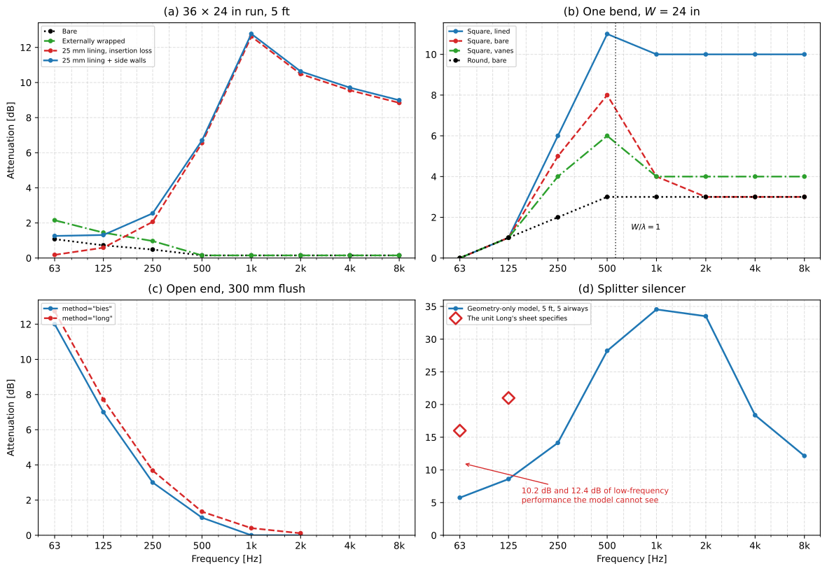
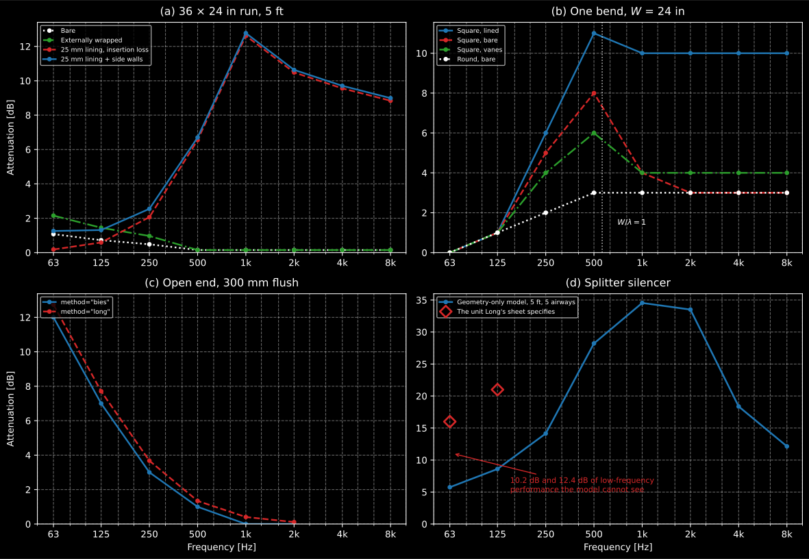
Four families, four different jobs. Lining a run changes the order of magnitude in the mid bands and does nothing at 63 Hz; a wrapped bare duct does the opposite, and both are useless above 1 kHz. The elbow tables are keyed on $W/\lambda$, which is why the same bend behaves alike in ducts of different size one octave apart. The two end-reflection methods agree within a decibel over the bands both cover, so the choice between them is not worth an argument. And the splitter panel is the honest one: the geometry-only regression cannot see the 10 to 12 dB of low-frequency performance a real low-frequency unit is designed for, which is why that row comes from a datasheet.

Show the code for this figure

import matplotlib.pyplot as plt

# `bands`, IN and FT as above; every model returns an HvacSpectrumResult.

# One line for one element:
lined_rectangular_duct_attenuation(bands, 36 * IN, 24 * IN, 5 * FT, 1 * IN,
                                   include_unlined=True).plot()
plt.show()

# By hand: the bend family of panel (b), keyed on W / lambda.
fig, ax = plt.subplots()
for label, kwargs in (("Square, lined", dict(bend_type="square", lined=True)),
                      ("Square, bare", dict(bend_type="square")),
                      ("Square, vanes", dict(bend_type="square", vanes=True)),
                      ("Round, bare", dict(bend_type="round"))):
    el = elbow_insertion_loss(bands, 24 * IN, **kwargs)
    ax.semilogx(el.frequencies, el.values, "o-", label=label)
ax.set_xlabel("Frequency [Hz]"); ax.set_ylabel("Insertion loss [dB]")
ax.legend()
plt.show()

One condition travels with the lined-elbow column and is easy to lose: the tables assume the duct lining extends at least three duct diameters up- and downstream of the bend, so lined=True describes a lined run that contains a bend rather than a lined bend in a bare duct. A bend in bare duct takes the unlined column; taking the lined one instead overstates the attenuation by the whole tabulated increment, 10 dB in the mid bands for the square bend above.

4. What the system puts back

Attenuation is only half the sheet. Every disturbance of the airflow generates noise of its own, and past a certain velocity the silencer bought to remove the fan becomes the loudest thing in the duct.

silencer_self_noise is Fry’s estimate as Long Eq. 14.31,

$$L_W=55{\log }_{10}\frac{V}{V_0}+10{\log }_{10}N+10{\log }_{10}\frac{H}{H_0}-45,$$

spread over the octave bands by the corrections of Table 14.8. The exponent is the whole message: the fifth-and-a-half power of the airway velocity means that doubling the face velocity of a silencer adds about 17 dB.

from phonometry import silencer_self_noise
import numpy as np

IN = 0.0254
slow = silencer_self_noise(None, airway_velocity=10.0, passages=5,
                           height=24 * IN)
fast = silencer_self_noise(None, airway_velocity=20.0, passages=5,
                           height=24 * IN)
print(np.round(slow.values, 1))
# [40.8 40.8 38.8 36.8 31.8 26.8 21.8 16.8]
print(round(float(fast.values[0] - slow.values[0]), 1))     # 16.6 dB

Straight duct and bends regenerate too, through flow_noise_straight_duct and flow_noise_bend (VDI 2081 as Bies Eqs. (8.251) and (8.254)); the bend model carries the Strouhal-number transition from the sixth-power inner-corner dipole to the eighth-power outer-corner quadrupole.

The terminal device is the last one in the path and the one nothing downstream can fix, because there is no ductwork left after it. Its sound power is normally manufacturer data measured to ASHRAE Standard 70, and that is what a real sheet uses. When there is none to hand, diffuser_sound_power is Reynolds’s estimate as Long Eqs. 13.27 to 13.33: an overall level $L_W=10{\log }_{10}{S}_G+30{\log }_{10}\xi +60{\log }_{10}{U}_G-31.3$ from the face area $S_G$, the approach velocity $U_G=Q/S_G$ and the normalised pressure-drop coefficient $\xi =334.9\Delta p/({\rho }_0{U}_G^2)$ of Eq. 13.28. Long writes all four in foot-pound units ($S_G$ in ft², $U_G$ in ft/s, $\Delta p$ in inches of water gauge); diffuser_sound_power takes and returns SI and converts internally, which is why the constants here are quoted on Long’s units. The spectrum follows as $L_{W,\text{oct}}=L_W+C_D$ with the shape function $C_D=-11.82-0.15A-1.13A^2$ for a rectangular device ($-5.82$ for a round one), where $A$ is the distance in octaves from the peak band $f_P=48.8U_G$ (Eq. 13.32, $U_G$ in ft/s), counted on Long’s band numbering with band 0 at 32 Hz.

from phonometry import diffuser_sound_power
import numpy as np

IN, CFM, IN_WG = 0.0254, 0.0004719474432, 249.0

# The supply diffuser of Long's worked sheet: 24 x 24 in, 312 cfm, 0.05 in pd.
print(np.round(diffuser_sound_power(None, (24 * IN) ** 2,
                                    volume_flow=312 * CFM,
                                    pressure_drop=0.05 * IN_WG).values, 1))
# [ 33.4  32.4  29.1  23.6  15.9   5.9  -6.4 -21. ]
# Long Table 14.9 prints 33/32/29/23/15/4/0/0 for that row.

# The peak band the shape function is counted from, on Long's units:
face_velocity = 312 * CFM / (24 * IN) ** 2 / 0.3048   # 1.3 ft/s
print(round(48.8 * face_velocity, 1))                 # fP = 63.4 Hz
print(round(np.log2(48.8 * face_velocity / 32.0)))    # band 1: the 63 Hz octave

The sixth power of velocity in Eq. 13.27 is the design rule: about 18 dB per doubling of the approach velocity once the pressure drop follows it, and about 15 dB back for every doubling of face area at the same air volume. Two screening rules from ASHRAE Chapter 49 come with it. air_terminal_velocity_limit (Table 9) gives the maximum neck velocity for a design RC, and air_terminal_damper_correction (Table 10) gives the penalty for throttling a balancing damper, which is where a great many finished installations fail.

from phonometry import air_terminal_damper_correction, air_terminal_velocity_limit

print(air_terminal_velocity_limit(30, opening="supply"))   # 2.2 m/s
print(air_terminal_velocity_limit(30, opening="return"))   # 2.5 m/s
print(air_terminal_damper_correction(3.0, location="diffuser_neck"))  # 15.0 dB
print(air_terminal_damper_correction(3.0, location="supply_duct"))    #  2.0 dB

Fifteen decibels in the neck against two decibels 1.5 m back in the duct, for the same pressure ratio, is the entire design rule: throttle far from the outlet, or balance the system by sizing the ductwork instead.

Both of this section’s models are governed by a slope, and slopes are what figures are for.

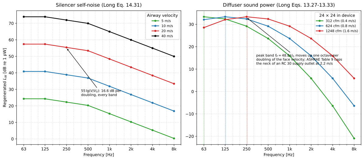
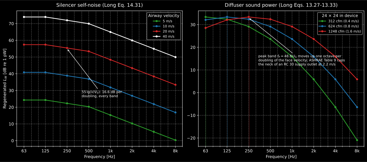
The two exponents, drawn. The silencer’s is the harsher: 55 lg of the airway velocity puts four parallel curves 16.6 dB apart for every doubling, in every band at once, which is why a silencer sized for pressure drop rather than for face velocity becomes the loudest element in the run. The diffuser’s peak band moves as well as its level — $f_P=48.8U_G$ in Long’s units — so a faster outlet is not simply louder, it moves its noise into the bands a criterion curve judges most harshly. The crossing that matters on a real sheet is where one of these curves meets the attenuated fan level: past it, the element bought to solve the problem is the problem.

Show the code for this figure

import matplotlib.pyplot as plt

# `silencer_self_noise` and `diffuser_sound_power` as imported above.
bands = [63.0, 125.0, 250.0, 500.0, 1000.0, 2000.0, 4000.0, 8000.0]

# One line for one element:
silencer_self_noise(bands, airway_velocity=20.0, passages=5,
                    height=24 * IN).plot()
plt.show()

fig, ax = plt.subplots()
for velocity in (5.0, 10.0, 20.0, 40.0):
    res = silencer_self_noise(bands, airway_velocity=velocity, passages=5,
                              height=24 * IN)
    ax.semilogx(res.frequencies, res.values, "o-", label=f"{velocity:.0f} m/s")
ax.set_xlabel("Frequency [Hz]"); ax.set_ylabel("Regenerated L_W [dB re 1 pW]")
ax.legend()
plt.show()

4.1 The path that is not in the sheet: breakout

The cascade above accounts only for what stays inside the duct. A duct crossing an occupied space is also a radiating surface, and ASHRAE HVAC Applications Chapter 49 states that transmission below 250 Hz through duct breakout is often a major acoustical limitation. The power leaving through the walls is

$$L_{W,\text{out}}=L_{W,\text{in}}+10{\log }_{10}(S/A)-{\mathrm{TL}}_{\text{out}},$$

with $S=2L(a+b)$ the radiating surface area of a rectangular duct and $A=ab$ its cross-section. For this page’s own 36 × 24 in trunk over a 3 m run that geometric term is $10{\log }_{10}[2\times 3\times (0.914+0.610)/(0.914\times 0.610)]=12.1$ dB, so a wall transmission loss in the teens puts the radiated power within a few decibels of what is still inside the duct.

The exposure is worst exactly where the sheet still has all its level: at low frequency, and in the first metres after the fan, before any silencer. A reader can complete this sheet, pass NC 30, and still fail the room on rumble radiated by the trunk crossing the ceiling void — the sheet cannot see it, because breakout leaves the path the sheet is walking. The design rules that follow are short: get the attenuation in before the duct crosses the space, prefer round or dual-wall duct and a radiused discharge take-off over a high-aspect-ratio rectangular trunk, and treat lagging as a last resort rather than a fix, because lagging a rectangular duct is often ineffective. Nothing in this library models breakout; it is named here so that it is not forgotten.

5. From sound power to room level

The last step converts the sound power arriving at the terminal device into a sound pressure level where somebody is sitting, through the steady-state room relation $L_p=L_W+10{\log }_{10}\left[Q/(4\pi r^2)+4/R\right]$. room_effect returns that as a positive attenuation so it drops into the cascade beside every other loss, with $Q=2$ by default for a diffuser flush in a ceiling.

from phonometry import room_constant, room_effect

# The 20 x 20 x 8 ft room of Long's worked sheet, drywall and carpet.
area = 2 * 6.10 * 6.10 + 4 * 6.10 * 2.44        # 134.0 m2
r_const = room_constant(area, 0.15)             # 23.6 m2
print(round(float(room_effect(1.83, r_const, directivity=2.0)), 1))   # 6.6 dB

Long’s sheet prints 5 to 7 dB for that room across the bands, so a single mean absorption of 0.15 lands in the right place; a per-band absorption gives a per-band room effect, which is what the carpet actually does.

Three of the four inputs deserve naming. The distance is the straight line from the terminal device to the listener’s head, and 1.83 m is the 6 ft Long uses for a seated occupant under a ceiling diffuser; halving it costs 6 dB in the direct term only, which is why the room effect flattens out once the reverberant term takes over. The directivity $Q$ is 2 for a device flush in one surface, 4 where a wall meets the ceiling and 8 in a corner, because a grille in a corner puts its power into an eighth of the sphere. And the formula is written for one source: a room served by four diffusers each carrying a quarter of the flow is roughly $10{\log }_{10}4=6$ dB louder at a point equidistant from them than a single-diffuser sheet predicts. The honest calculation runs one path per outlet and combines them with combine_duct_paths, exactly as the supply and return paths are combined in section 6. Several outlets over one listener is the commonest reason a passing sheet fails on site.

5.1 The verdict: criterion curve, exceedance and rating

Pass target= and criterion= to duct_path and the result rates itself. criterion_curve samples the NC or RC curve at the analysis bands, exceedance is the band-by-band excess over it, meets_target is the band-by-band verdict a design sheet applies, and rating is the full NCResult or RCResult derived by the ANSI/ASA S12.2-2019 procedure, which is a different question and can differ from the tangency verdict. A spectrum can rate NC-27 and still poke through the NC 30 curve in one band, because the standard’s designation procedure and a sheet’s “no band above the curve” are different questions; meets_target answers the second.

That distinction has to be settled before the job is built, because the design verdict and the commissioning verdict must be the same quantity. An acceptance test specifies: every terminal device serving the space running at the design flow with the balancing dampers in their final positions — which is where the 15 dB neck penalty of air_terminal_damper_correction actually shows up, and it is not in any design sheet; microphone positions in the occupied zone rather than under a diffuser; the system switched off to establish the background level, with the correction rule agreed in advance; and the rating procedure applied to the measured octave-band spectrum rather than read off by tangency. Write into the specification whichever verdict is going to be measured — band-by-band against the curve, or the S12.2 rating — and not one for the design and the other for the test. Room-noise criteria has the rating procedure itself.

6. The worked example: Long’s Table 14.9

Long’s Chapter 14 closes with a complete sheet: a 5000 cfm forward-curved fan at 2 in w.g., feeding one room through a supply path (elbow, silencer, lined duct, a 25 per cent branch split, a second lined duct, flexible duct, a rectangular diffuser) and a return path (elbow, low-frequency silencer, lined elbow, plenum, grille), each ending in the room effect of a 20 x 20 x 8 ft carpeted office, combined and checked against NC 30. Every row below is the one Long prints, including the manufacturer data for the silencers and the terminal devices, which is what a real sheet uses.

Thirteen rows of a table are hard to hold in the head; the same thirteen rows as a building are not.

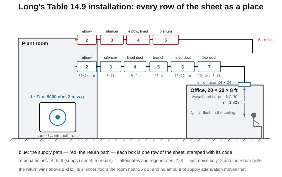
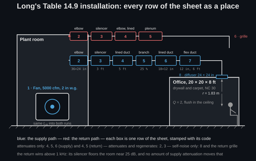
The sheet as a place. The two runs start from the same fan row because a fan radiates the same power from its intake and its discharge; the codes on the boxes are the code= strings the snippet below stamps on each DuctElement, so a row that fails in the table can be pointed at in the building. The last line of the legend is the answer this whole sheet arrives at, before any arithmetic: the return path, not the supply, is what the office hears above 1 kHz.

import numpy as np
from phonometry import DuctElement, combine_duct_paths, duct_path

bands = [63.0, 125.0, 250.0, 500.0, 1000.0, 2000.0, 4000.0, 8000.0]
fan = [90.0, 86.0, 82.0, 79.0, 77.0, 75.0, 71.0, 61.0]
source = "Fan, centrifugal FC, 5000 cfm, 2 in w.g."

supply = duct_path(
    bands, fan,
    [
        DuctElement("Elbow, 36 x 24 in, unlined", [0, 1, 2, 3, 3, 3, 3, 3],
                    [41, 39, 36, 29, 20, 6, 0, 0], code="2"),
        DuctElement("Silencer, 3 ft, standard pressure drop",
                    [7, 12, 16, 28, 35, 35, 28, 17],
                    [49, 43, 44, 42, 42, 45, 35, 24], code="3"),
        DuctElement("Duct, 36 x 24 in, 5 ft, 1 in lining",
                    [2, 2, 3, 7, 15, 12, 11, 9], code="4"),
        DuctElement("Split, 25 per cent", 6.0, code="5"),
        DuctElement("Duct, 18 x 12 in, 6 ft, 1 in lining",
                    [3, 3, 5, 11, 25, 22, 16, 13], code="6"),
        DuctElement("Flexible duct, 12 in, 6 ft",
                    [14, 14, 16, 15, 17, 22, 16, 13], code="7"),
        DuctElement("Rectangular diffuser, 312 cfm", None,
                    [33, 32, 29, 23, 15, 4, 0, 0], code="8"),
    ],
    room_effect=[6, 6, 5, 5, 6, 7, 6, 6],
    source_label=source, target=30.0, label="Supply",
)

ret = duct_path(
    bands, fan,
    [
        DuctElement("Elbow, 36 x 24 in, unlined", [0, 1, 2, 3, 3, 3, 3, 3],
                    [43, 42, 39, 33, 24, 12, 0, 0], code="2"),
        DuctElement("Silencer, 5 ft, low-frequency type",
                    [16, 21, 35, 41, 41, 28, 21, 15],
                    [51, 49, 53, 56, 56, 59, 60, 53], code="3"),
        DuctElement("Elbow, 36 x 24 in, lined, 1 in", [1, 2, 3, 4, 5, 6, 8, 10],
                    [39, 38, 34, 28, 18, 4, 0, 0], code="4"),
        DuctElement("Plenum, 800 sq ft, 50 per cent lined",
                    [12, 13, 19, 20, 20, 20, 21, 21], code="5"),
        DuctElement("Rectangular grille, 24 x 24 in, 563 cfm", None,
                    [30, 29, 26, 20, 12, 1, 0, 0], code="6"),
    ],
    room_effect=[9, 8, 6, 8, 8, 8, 9, 10],
    source_label=source, target=30.0, label="Return",
)

total = combine_duct_paths([supply, ret], label="Supply + return")
print(np.round(supply.received_level, 0))    # Long: 52 42 30 18  9 -2 -2 -1
print(np.round(ret.received_level, 0))       # Long: 52 41 27 25 23 25 22 12
print(np.round(total.received_level, 0))     # Long: 55 45 32 26 23 25 22 12
print(total.meets_target)                    # True
print(round(float(total.rating.rating), 1))  # 26.7, governed at 63 Hz

Every printed row comes back within the sheet’s own 1 dB rounding: the supply is 1 dB low at 4 kHz, the return 1 dB low at 500 Hz, and the combination 1 dB low at 500 Hz and 1 dB high at 8 kHz, everything else exact. The room lands at NC 27, comfortably inside its NC 30 target, and the 63 Hz band is what governs the rating, which is the usual outcome of a duct-noise design and the reason low-frequency silencer performance is worth paying for.

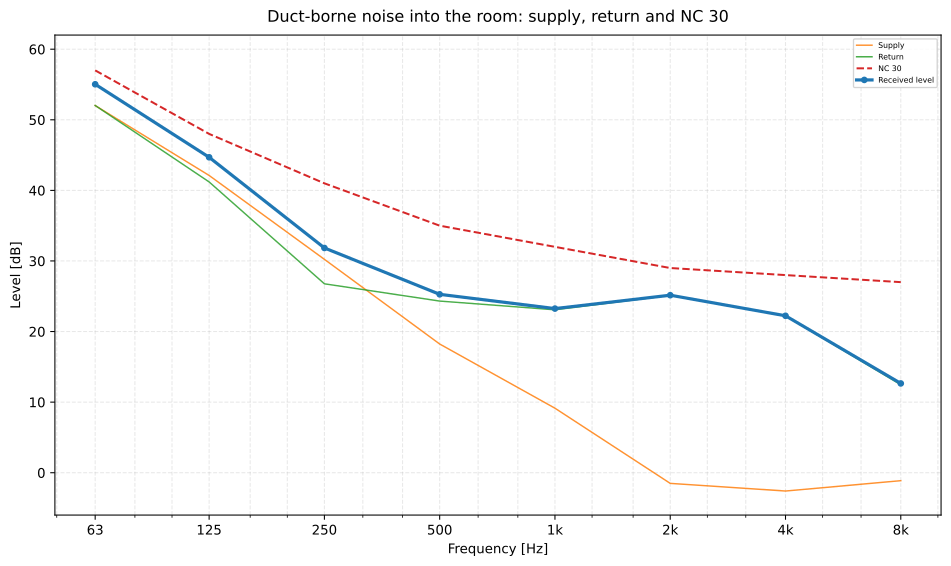
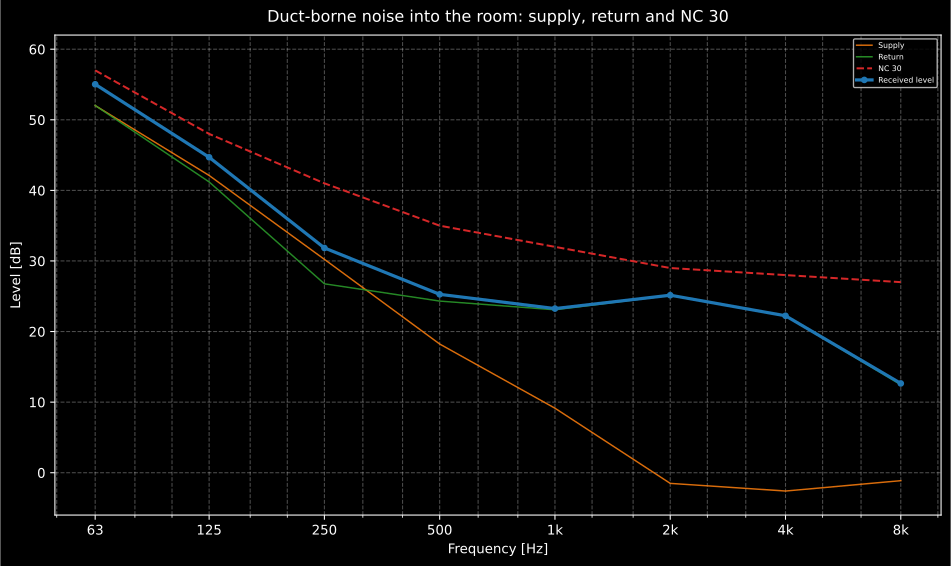
The two paths and their sum against NC 30. The supply, with its silencer, two lined runs, a branch split and six feet of flexible duct, has nothing left above 1 kHz; the return, with a plenum but a silencer whose own self-noise floors it near 25 dB, is what the room actually hears in the mid and high bands. Adding low-frequency attenuation to the supply would change nothing at all: the return already sets the answer everywhere except at 63 Hz, and that is the row to argue about.

Show the code for this figure

import matplotlib.pyplot as plt
from phonometry import combine_duct_paths

# `supply` and `ret` are the two DuctPathResult objects built above.

# One line for one path: the cascade of the supply run against NC 30.
supply.plot()
plt.show()

# The concept figure: both paths, their energy sum and the criterion.
total = combine_duct_paths([supply, ret], label="Supply + return")
total.plot()
plt.gca().set_ylim(-6.0, 62.0)
plt.show()

DuctPathResult also prints and files itself. .table() returns the sheet row by row with the worksheet sign convention, and .report() renders a one-page PDF in the layout of the published procedures (AHRI Standard 885 Table 8; Long Table 14.9): the element table, the cascade chart against the criterion curve, the boxed room-criterion rating and the verdict.

for row in total.table():
    print(f"{row['kind']:<12} {row['label'][:26]:<26} "
          f"{[round(float(v)) for v in row['values']]}")

supply.report("duct-path-supply.pdf")    # the fiche previewed below
total.report("duct-path.pdf")            # the combination; needs phonometry[report]

The example fiche is the supply half of the sheet, regenerated with make reports and kept rendered in the repository. Click the preview to open the PDF:

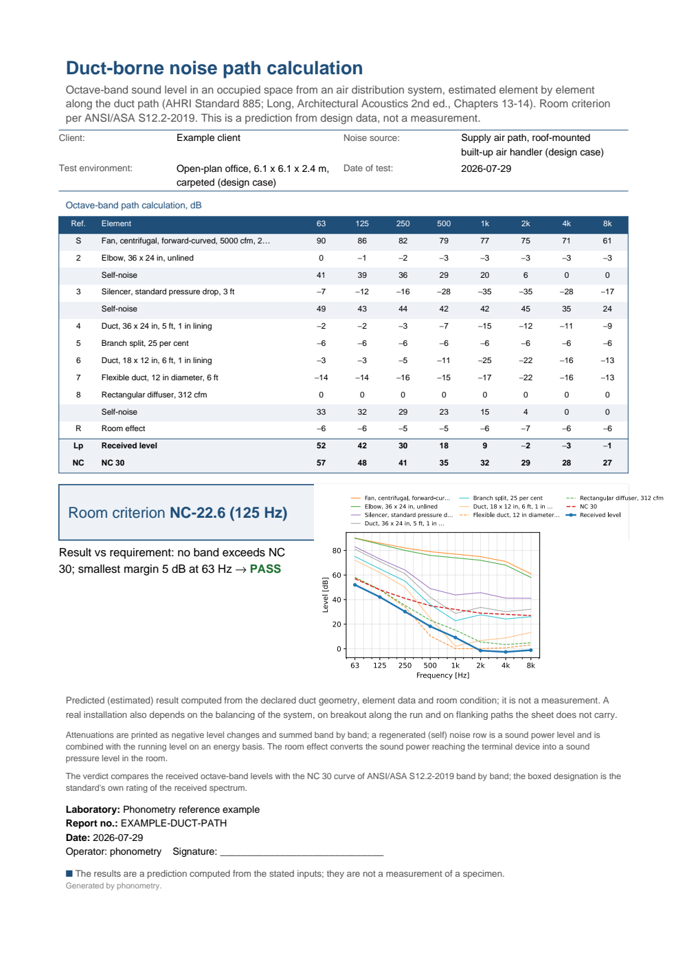
Duct-borne noise path calculation example report: a metadata header with the client, the noise source, the test environment and the date, the octave-band path table listing the fan sound power, each element attenuation as a negative level change, the self-noise rows of the elbow, the silencer and the diffuser, the room effect, the received level and the NC 30 curve, and beneath it the boxed room criterion NC-22.6 at 125 Hz with the verdict that no band exceeds NC 30 beside the cascade chart of every element against the criterion curve.

Download the report (PDF)

Duct-borne noise path fiche (DuctPathResult.report): the supply path of the worked sheet element by element, rated NC-22.6, governed at 125 Hz, and passing its NC 30 target in every band.

7. What reproduces, and what does not

Long’s Table 14.9 was produced by a commercial computer program, not by hand from the tables printed alongside it, and being honest about that is more useful than pretending otherwise. The arithmetic of the sheet is reproduced exactly, as section 6 shows. Several of its element rows, however, do not follow from the book’s own printed data, and the functions in this library implement the printed equations and tables. Verified band by band:

• The fan row does not come from Eq. 13.1. The sheet prints 90/86/82/79/77/75/71/61 dB. Eq. 13.1 with the Table 13.5 forward-curved constants at 5000 cfm and 2 in w.g. gives 99/99/89/84/82/77/72/67 dB, and the printed spectrum is not a level shift of the tabulated one, so it comes from other data (a manufacturer’s, most likely).
• The flexible-duct row is not Table 14.4. The sheet prints 14/14/16/15/17/22/16/13 dB for 12 in by 6 ft; flexible_duct_insertion_loss reads 3/5/10/15/17/16/9 dB out of the table for that duct.
• The lined rectangular ducts agree in the mid and high bands. For the 18 x 12 in, 6 ft, 1 in run the library returns 11/25/22/16/13 dB from 500 Hz up, exactly the printed row, and is 1 to 2 dB high below it (5/4/6 against 3/3/5). For the 36 x 24 in, 5 ft run it matches at 250, 500 and 8 kHz and is 1 to 2 dB low elsewhere.
• The split and the unlined elbow reproduce exactly. split_loss gives the 25 per cent branch as 6.0 dB against the printed -6 dB, and elbow_insertion_loss gives 0/1/2/3/3/3/3/3 dB against the printed row when the elbow is read as round (Table 14.7) at $w=24$ in.
• The supply diffuser row reproduces too. diffuser_sound_power on a 24 x 24 in rectangular device at 312 cfm and 0.05 in pd returns 33.4/32.4/29.1/23.6/15.9/5.9 dB against the printed 33/32/29/23/15/4, inside the sheet’s own rounding in the five bands that carry the level. The return grille row (30/29/26/20/12/1) does not follow from the same equations at its 563 cfm, so it is manufacturer data.
• The NC 30 row differs by 1 dB at 1 kHz. Long prints 57/48/41/35/31/29/28/27; the library’s nc_curve(30) returns 57/48/41/35/32/29/28/27, the values of ANSI/ASA S12.2-2019 Table 1. Long is using the original Beranek 1957 curve. The difference does not change the verdict here, but it is worth knowing which NC you are quoting.

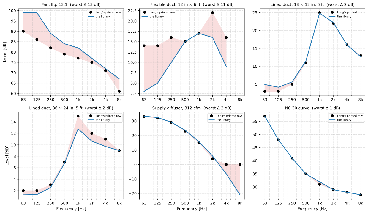
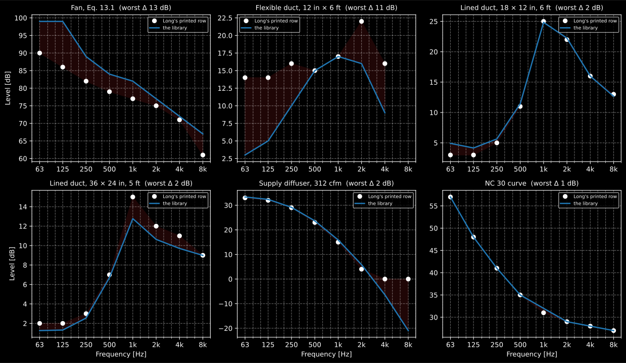
Where the sheet is a calculation and where it is a datasheet, seen at a glance. The two lined runs and the diffuser sit inside the sheet’s own rounding, so those rows really are the printed equations. The fan and the flexible duct do not, and the shape of the disagreement says why: the fan’s printed spectrum is not a level shift of the tabulated one, so it comes from other data, and the flexible-duct row is far above ASHRAE Table 14.4 at low frequency, which is where its breakout lives. The last panel is the one to remember when quoting a rating: Long’s NC 30 is the original Beranek 1957 curve and differs from ANSI/ASA S12.2-2019 Table 1 by 1 dB, in the 1 kHz band alone.

Show the code for this figure

import matplotlib.pyplot as plt

# Every model is imported above; nc_curve returns the 10-band curve aligned
# with OCTAVE_BANDS, which starts at 16 Hz, so the sheet's eight bands are
# nc_curve(30)[2:].
printed = [3, 3, 5, 11, 25, 22, 16, 13]      # Long's 18 x 12 in, 6 ft row
computed = lined_rectangular_duct_attenuation(
    bands, 18 * IN, 12 * IN, 6 * FT, 1 * IN, include_unlined=True).values

fig, ax = plt.subplots()
ax.fill_between(bands, printed, computed, alpha=0.25)
ax.semilogx(bands, printed, "o", label="Long's printed row")
ax.semilogx(bands, computed, "-", label="the library")
ax.set_xlabel("Frequency [Hz]"); ax.set_ylabel("Level [dB]")
ax.legend()
plt.show()

None of that is a defect of the sheet. It is what a real duct-borne calculation looks like: the elements a manufacturer publishes (fans, silencers, diffusers, grilles) come from test data, and the elements nobody publishes (duct runs, elbows, splits, end reflections, the room) come from the tables. DuctElement takes both without caring which is which, which is the point.

8. The plane-wave limit

Every element model above, and every four-pole silencer in Silencers, is one-dimensional. It assumes a single sound pressure describes the whole duct cross section, which is true only below the frequency at which the first higher-order acoustic mode cuts on. Above it several modes propagate at once, each with its own axial wavenumber, and a plane-wave prediction quietly stops being right.

noise_control.duct_modes implements the cut-on analysis of Norton & Karczub, Fundamentals of Noise and Vibration Analysis for Engineers (2nd ed.), section 7.3: circular ducts by Eq. 7.6 with the $\pi {\alpha }_{pq}$ eigenvalues of Table 7.1 that solve $J_p^{\prime }({\kappa }_{pq}{a}_i)=0$, rectangular ducts by Eq. 7.10,

$$(f_{\text{co}}{)}_{pq}=\frac{c}{2}\sqrt{(p/a{)}^2+(q/b{)}^2}\sqrt{1-M^2},$$

and the mean-flow correction of Eqs. 7.8 and 7.9, in which a uniform axial flow of Mach number $M$ lowers every cut-on frequency by $\sqrt{1-M^2}$ and moves the cut-on itself from $k_x=0$ to $k_x=-M{\kappa }_{pq}/\sqrt{1-M^2}$.

import numpy as np
from phonometry import plane_wave_limit, rectangular_duct_cut_on

# Norton problem 7.2: a 0.65 x 0.4 m air-conditioning duct at 15 m/s.
modes = rectangular_duct_cut_on(0.65, 0.40, flow_velocity=15.0, count=6)
print(modes.modes[:3])                          # ((1, 0), (0, 1), (1, 1))
print(np.round(modes.cut_on[:3], 1))            # [263.6 428.3 502.9] Hz
print(np.round(modes.cut_on_no_flow[:3], 1))    # [263.8 428.8 503.4] Hz
print(round(modes.plane_wave_limit, 1))         # 263.6 Hz

IN = 0.0254
print(round(plane_wave_limit(width=36 * IN, height=24 * IN), 1))   # 187.6 Hz
print(round(plane_wave_limit(diameter=12 * IN), 1))                # 659.5 Hz

Those ventilation numbers are blunt: in that duct plane waves are the whole story only up to the 250 Hz octave, and a 36 x 24 in supply trunk gives up at 188 Hz.

What a number cannot say is that cut-on is a switch, not a slope. The clip below simulates the 0.65 m dimension of that same duct as a 2D slice, rigid walls, and drives it twice with one off-axis source that excites the plane mode and the first transverse mode together — once at 180 Hz, below the 263.8 Hz the snippet just printed, and once at 400 Hz above it. Nothing else differs. Below cut-on the transverse mode is evanescent: it decays as $e^{-\alpha x}$ with $1/\alpha =0.28$ m, which puts it 20 dB down 0.65 m from the source — one duct width — so the lumpy near field dies there and every wavefront after it crosses the section flat. Above cut-on it propagates, the two modes run at different axial wavenumbers ($k_x=5.51$ against $k=7.33$ rad/m at 400 Hz) and beat along the duct every 3.45 m, and the profile across the section never settles. The panel beside each strip draws that profile at a fixed station 5 m downstream against its own section average — which is the single pressure the one-dimensional models above carry — so “a single sound pressure describes the whole cross section” is either true on screen or visibly false.

The same 0.65 metre rigid duct is driven at 180 Hz and at 400 Hz by one off-axis source. In the 180 Hz strip the lumpy field near the source flattens within half a duct width and every later wavefront crosses the section as a straight line, and the profile panel beside it collapses onto its own average. In the 400 Hz strip the field stays lumpy the whole length of the duct, the two propagating modes beat along it, and the profile panel swings far away from the average on every cycle.

Download the animation (WebM)

The same 0.65 metre rigid duct is driven at 180 Hz and at 400 Hz by one off-axis source. In the 180 Hz strip the lumpy field near the source flattens within half a duct width and every later wavefront crosses the section as a straight line, and the profile panel beside it collapses onto its own average. In the 400 Hz strip the field stays lumpy the whole length of the duct, the two propagating modes beat along it, and the profile panel swings far away from the average on every cycle.

Download the animation (WebM)

That is why a transfer-matrix silencer model has a ceiling frequency rather than an accuracy budget: below cut-on the second mode is not small, it is absent, and above it the model is describing one of several waves that are all there. The Silencers four-pole algebra inherits the same limit.

At 15 m/s the flow correction is invisible: $M=0.044$ gives $\sqrt{1-M^2}=0.999$, which moves the first cut-on by 0.2 Hz. It earns its place in high-speed pipework instead. Norton’s problem 7.1 is that case, a 254 mm line carrying steam ($c=405$ m/s) at 200 m/s, $M=0.494$, and there the two ladders separate by more than a hundred hertz at every rung.

import numpy as np
from phonometry import circular_duct_cut_on

# Norton problem 7.1: a 254 mm circular duct carrying steam at 200 m/s.
steam = circular_duct_cut_on(0.254, flow_velocity=200.0,
                             speed_of_sound=405.0, count=6)
print(steam.modes)
# ((1, 0), (2, 0), (0, 1), (3, 0), (4, 0), (1, 1))
print(np.round(steam.cut_on_no_flow, 1))
# [ 934.5 1550.1 1944.7 2132.3 2698.9 2705.9]
print(np.round(steam.cut_on, 1))
# [ 812.6 1347.9 1691.1 1854.1 2346.8 2352.9]
print(np.round(steam.axial_wavenumber, 2))
# [ -8.23 -13.66 -17.13 -18.79 -23.78 -23.84]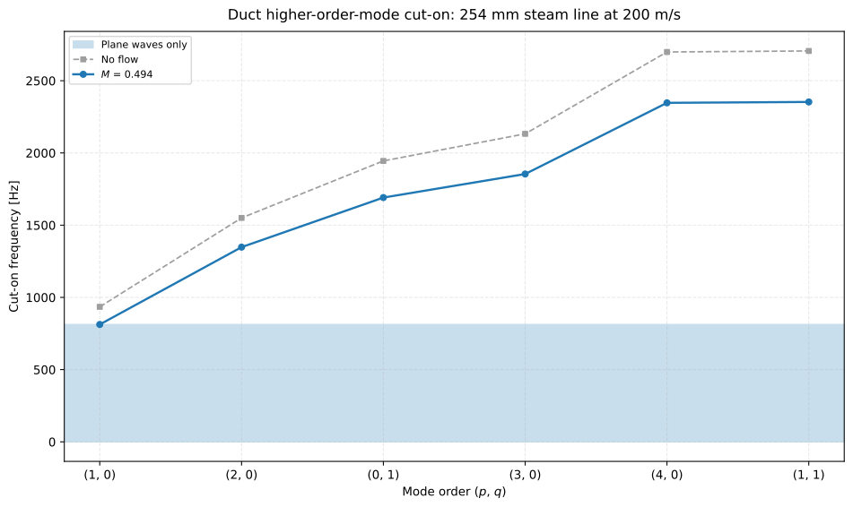

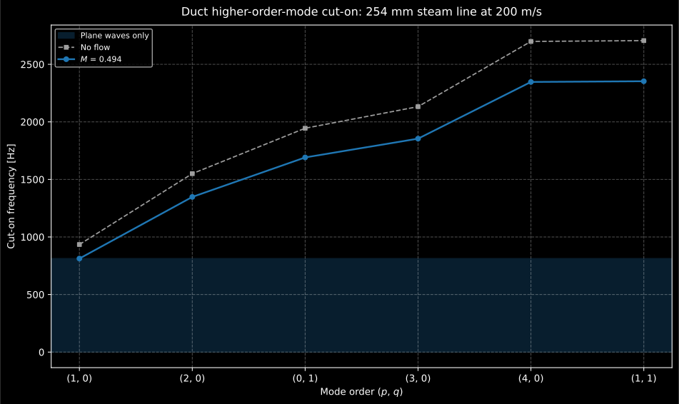
Norton’s problem 7.1, the case where the mean flow is worth drawing: half the speed of sound in the pipe pulls every cut-on down by $\sqrt{1-M^2}=0.870$, so the first higher-order mode appears at 813 Hz instead of 935 Hz and the plane-wave band, shaded, is 13 per cent narrower than the still-air calculation would promise. The axial wavenumber at cut-on is negative in every rung: with flow, the mode is already travelling upstream at the frequency at which it appears.

Show the code for this figure

import matplotlib.pyplot as plt
from phonometry import circular_duct_cut_on, rectangular_duct_cut_on

# One line for one duct: the cut-on ladder with the plane-wave band shaded.
steam = circular_duct_cut_on(0.254, flow_velocity=200.0,
                             speed_of_sound=405.0, count=6)
steam.plot()
plt.show()

# The ventilation duct of problem 7.2, where the flow shift is negligible.
rectangular_duct_cut_on(0.65, 0.40, flow_velocity=15.0, count=6).plot()
plt.show()

Two results carry this limit for you. Every ReactiveSilencerResult reports the first cut-on of its widest cross section as plane_wave_limit, and duct_path accepts a section= description of the duct it is walking. Both raise a PlaneWaveWarning when the analysis grid runs past that frequency: the numbers are still returned, and above cut-on they describe the plane-wave mode alone, which a measurement will not.

import warnings
from phonometry import DuctElement, PlaneWaveWarning, duct_path

IN = 0.0254
bands = [63.0, 125.0, 250.0, 500.0, 1000.0, 2000.0, 4000.0, 8000.0]

with warnings.catch_warnings(record=True) as caught:
    warnings.simplefilter("always")
    duct_path(bands, [90.0] * 8, [DuctElement("Straight run", 3.0)],
              section={"width": 36 * IN, "height": 24 * IN},
              flow_velocity=6.0, label="Supply")
print(caught[0].category is PlaneWaveWarning)
print(str(caught[0].message))
# Supply: 6 of 8 frequencies are above the first duct cut-on frequency
# (188 Hz), where higher-order modes propagate and the plane-wave result
# describes the plane-wave mode only.

Six of the eight octave bands of a standard duct-noise sheet sit above the cut-on of a 36 x 24 in duct. That is not a reason to distrust the sheet: the ASHRAE element models it is built from are empirical, fitted to measurements of real ducts in which those modes were present, so they carry the multimode behaviour inside their regression constants. The warning is aimed at the analytical methods, the four-pole silencer algebra above all, where the plane-wave assumption is structural rather than statistical, and where the peaks and troughs of a computed transmission loss simply do not survive past cut-on.

What this guide covers

• Covered

  The fan source model (fan_sound_power, fan_efficiency_correction, blade_passing_frequency, fan_casing_attenuation; Long Eq. 13.1 with Tables 13.5-13.8); the run attenuations (lined and unlined rectangular and circular ducts, flexible_duct_insertion_loss, elbow_insertion_loss, split_loss, end_reflection_loss in both published methods, splitter_silencer_insertion_loss, plenum_attenuation); the regenerated noise (silencer_self_noise, flow_noise_straight_duct, flow_noise_bend, diffuser_sound_power and the ASHRAE Chapter 49 screening rules air_terminal_velocity_limit and air_terminal_damper_correction); room_effect and the criterion machinery; the cascade itself (duct_path, combine_duct_paths, .table(), .report()); and the duct_modes cut-on analysis.

• Not covered

  No fan or terminal-device data is predicted where the manufacturer publishes it, and this sheet expects the published figure. There is no dissipative-liner model: the splitter estimate is a lined-duct regression and the plenum attenuation is Wells’ closed form. Above the first cut-on the element models stand on their empirical fit alone. And four noise paths of a real installation are outside this calculation entirely, which is why a passing sheet and a failing room are usually one of them:

  • Duct breakout, treated in section 4.1: a large low-frequency-carrying trunk radiating through its own walls into a space it merely crosses, frequently the governing path near a plant room.
  • Duct break-in and crosstalk: two rooms served by the same run hearing each other through it, regardless of the partition between them.
  • Structure-borne transmission of fan vibration through hangers, plinths and the slab, which no airborne sheet can see and which is treated with isolators, and whose dynamic transfer stiffness is measured in Transfer stiffness (ISO 10846).
  • The octave-band resolution itself, which averages a blade-passing tone into its band and so understates how a pure tone will be judged.

See also

• Silencers: the reactive four-pole elements (expansion chambers, Helmholtz, quarter-wave and extended-tube resonators) whose validity ends at the same cut-on frequency.
• Industrial noise control: the rest of the installation, the individual HVAC duct methods and machine-enclosure insertion loss.
• Room-noise criteria (NC / RC Mark II): the ANSI/ASA S12.2-2019 families the received spectrum is judged against.
• Steady-state room field: the room constant behind the room effect and the plenum reverberant term.
• API reference: noise_control.duct_path, noise_control.duct_modes, noise_control.hvac.

References

• Air-Conditioning, Heating and Refrigeration Institute. (n.d.). Procedure for estimating occupied space sound levels in the application of air terminals and air outlets (AHRI Standard 885). The industry row structure of the duct-borne calculation sheet (Table 8) that DuctPathResult.table() and .report() follow.
• American Society of Heating, Refrigerating and Air-Conditioning Engineers. (2019). ASHRAE handbook: HVAC applications (SI edition), Chapter 49, Noise and vibration control. ASHRAE. The air terminal velocity limits (Table 9), the volume-damper corrections (Table 10) and the guidance that fan sound power is best taken from manufacturer test data.
• Bies, D. A., Hansen, C. H., & Howard, C. Q. (2017). Engineering noise control (5th ed.). CRC Press. https://doi.org/10.1201/9781351228152The end-reflection table (§8.13), the elbow insertion loss (§8.11), the reduction of a splitter muffler to lined ducts (§8.10.5, Eq. 8.241), the plenum chamber (§8.17) and the flow-generated noise of ducts and bends (§8.15).
• Long, M. (2014). Architectural acoustics (2nd ed.). Academic Press. The fan sound-power model (Ch. 13, Eq. 13.1 with Tables 13.5-13.8) and the diffuser self-noise model (Ch. 13, Eqs. 13.27-13.33), the duct attenuation, flexible duct, split loss, end reflection, silencer self-noise and room effect of Ch. 14, and the worked duct-borne sheet of Table 14.9 this guide is built around.
• Norton, M. P., & Karczub, D. G. (2003). Fundamentals of noise and vibration analysis for engineers (2nd ed.). Cambridge University Press. https://doi.org/10.1017/CBO9781139163927The higher-order acoustic modes of ducts, the cut-on frequencies of circular and rectangular cross sections and the mean-flow correction (§7.3, Eqs. 7.6-7.10).