Transfer stiffness of resilient elements (ISO 10846)

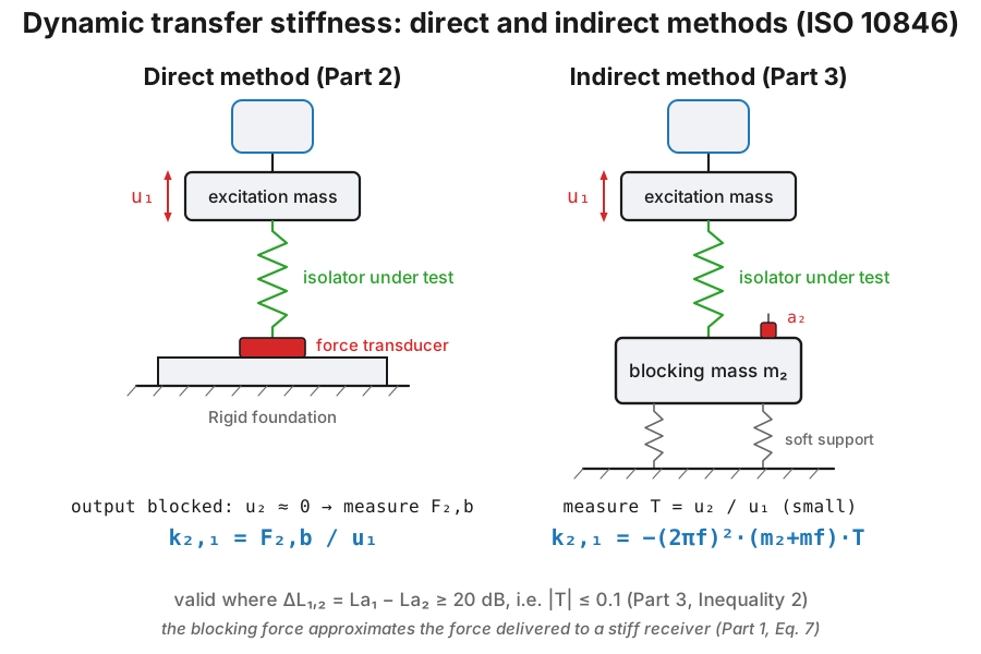
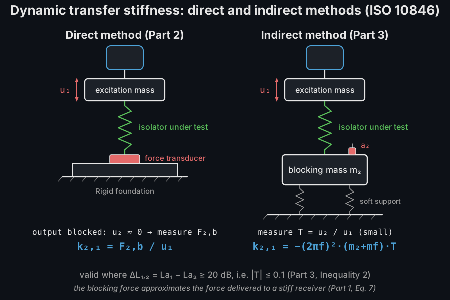
The vibro-acoustic transfer property of a resilient element (a vibration isolator, mount, bellows or hose) is its dynamic transfer stiffness $k_{2,1}$, the frequency-dependent ratio of the blocking force on the output (receiver) side to the displacement on the input (source) side (ISO 10846-1, 3.7):

Because a vibration isolator is only effective between structures of large driving-point stiffness, the force it delivers to the receiver approximates this blocking force (ISO 10846-1, Eq. 7), so $k_{2,1}$ is the quantity that characterises the isolator’s transmission. $k_{2,1}$ feeds the structure-borne source and building prediction standards: ISO 9611, EN 15657 and EN 12354-5.

The whole series is written around one bench, and it is the bench that says what the quantity means: the element is sandwiched between a driven input mass and an output that is either rigidly blocked or loaded with a known mass, under a stated static preload, and the two directions it is loaded in during service are measured separately.

Results are reported as a level re the reference stiffness $k_0=1\text{N/m}$ (ISO 10846-2 and -3, 3.17), and in the low-frequency range where inertial forces in the element are negligible the loss factor is the tangent of the phase angle of $k_{2,1}$ (ISO 10846-1, 3.8):

from phonometry import vibration

# A resilient mount with |k2,1| = 1 MN/m and a 5 % loss factor:
k = 1e6 * (1.0 + 0.05j)
print(round(float(vibration.transfer_stiffness_level(k)), 2))   # 120.01  dB re 1 N/m
print(round(float(vibration.loss_factor(k)), 3))                # 0.05

Why a blocked force rather than, say, the isolator’s transmissibility? Because a transmissibility is a property of a whole assembly: it changes with whatever masses and stiffnesses the isolator happens to connect, so data measured on one rig would not transfer to another installation. The blocked force per unit input displacement is a property of the element alone, and it predicts the force the element delivers to any receiver that is much stiffer than the element itself, which is exactly the situation a vibration isolator is designed for. ISO 10846 therefore sandwiches the isolator between a driven input mass and an output that is either rigidly blocked or loaded with a known mass (the rig drawn at the top of this page).

A transfer stiffness without its preload and its temperature is not a result. ISO 10846-1 clause 6.1 opens by saying so: $k_{2,1}$ depends on frequency, and “in addition, it is also dependent on static preload and, in many cases, on temperature”, and may depend on relative humidity as well. The laboratory conditions of every part of the series include the application of a static preload, because a rubber or spring isolator characterised unloaded is working at a different point on its load-deflection curve from the same isolator carrying its service load.

• Preload, applied and specified. ISO 10846-1 clause 6.3.3.1 gives the two rig topologies the diagram above draws. Gravity loading, where the output-side mass is the preload, is simple but unstable for large isolators at high preloads; a frame with an actuator (typically hydraulic) applies the load instead, with auxiliary springs decoupling the blocking mass from the frame, which is also what makes the indirect method less vulnerable to flanking transmission through the frame. Elements that are not resilient supports are loaded in the way their service demands: a static torque for a flexible coupling, a representative internal pressure for a bellows or hose (6.3.3.2).
• Creep. ISO 10846-2 clause 7.1: elements containing rubber-type components change load or deflection through creep, so the preload shall be applied to 100 % of the permissible static load, and the change of load or deflection due to creep should be less than 10 % per day before measurements begin.
• Temperature. ISO 10846-2 clause 7.6.1: measurements are made at one or more specified load conditions and temperatures covering the range met in practice; the temperature is monitored during the measurements; and the elements are exposed for at least 24 h to that temperature, within 3 °C, before testing.
• Contact and configuration. Clause 7.1 again: the element contacts the flanges over their whole surface (grease or double-sided tape helps, and large flanges may need flattening), and any device that is not part of the element in service is removed or de-activated.

Those conditions belong on the fiche of section 9 with the result: ReportMetadata carries them in its test_room and notes fields.

The direct method (ISO 10846-2) measures the blocked output force and the input displacement, $k_{2,1}=F_{2,\mathrm{b}}/u_1$. The indirect method (ISO 10846-3) loads the output with a compact blocking mass $m_2$ and measures the vibration transmissibility $T=u_2/u_1$; the blocking force is then the inertia force of the mass (ISO 10846-3, Eq. 1):

with $m_{\mathrm{f}}$ the mass of the output flange, which the flange_mass= keyword carries (it defaults to zero). It is not a refinement: ISO 10846-3 measures the vibration of the mass centre of the compact body formed by the blocking mass together with the output flange of the test element, so $m_{\mathrm{f}}$ is whatever is weighed with it: the flange and any auxiliary fixture that moves as part of the test element. Left at zero it reports a stiffness low by $m_2/(m_2+m_{\mathrm{f}})$. The approximation is valid well above the mass/spring resonance, where $T$ is small.

import numpy as np
from phonometry import vibration

# Indirect method: a 10 kg blocking mass, transmissibility 0.01 at 500 Hz,
# and the 1.2 kg output flange of the test element bolted on top of it.
k = vibration.transfer_stiffness_indirect(500.0, 0.01, blocking_mass=10.0,
                                          flange_mass=1.2)
print(f"{abs(complex(k)):.3e}")            # 1.105e+06  N/m
# flange_mass defaults to 0, which reports 9.870e+05 N/m: 12 % low here.

# Bundle a swept measurement into a result carrying its level and loss factor:
f = np.logspace(1.5, 3.3, 200)
t = vibration.base_transmissibility(f, mass=8.0, stiffness=1e6, damping=120.0)
res = vibration.indirect_transfer_stiffness_result(f, t, blocking_mass=8.0)
print(round(float(res.levels[-1]), 1))      # 125.1  dB re 1 N/m (high-f)

res.plot()   # the Lk(f) level spectrum, as in the figure above (needs matplotlib)

The TransferStiffnessResult carries the complex $k_{2,1}$ and exposes .levels, .loss_factor, .magnitude, .to("impedance"/"apparent_mass"), .band_average() (section 4) and .plot().

ISO 10846-1 clause 6.1 counts three methods, not two, “because they are complementary with respect to their strong and weak points”. The third is the driving-point method, which measures the input displacement and the input force and so yields the driving-point stiffness $k_{1,1}$ rather than $k_{2,1}$. Only at low frequencies, below the element’s first internal resonance, where the driving-point and transfer stiffnesses are equal, can it be used to determine the transfer stiffness, which is why the series covers it at all: owners of expensive driving-point rigs can use them for the low-frequency transfer stiffness. That same identity is why the fiche of section 9 boxes the low-frequency plateau rather than a value at one frequency: below the internal resonances there is only one stiffness to report. Part 5 of the series specifies that method, and section 6 below computes it, with the frequency up to which it may stand for the transfer stiffness.

The methods split the frequency axis between them, and the two limits of the indirect method have names. It is valid between $f_2$ and $f_3$, “typically 20 Hz $\le f_2\le$ 50 Hz and 2 kHz $\le f_3\le$ 5 kHz” (ISO 10846-3, clause 1), and the two are moved by opposite things:

• $f_2$ is where Inequality 2 starts to hold. Below it the rig’s own resonances (the element, the load-distribution plate, the blocking mass and the auxiliary springs together) break the impedance mismatch. It sits at roughly three times the highest natural frequency of that assembly, and a heavier blocking mass lowers it.
• $f_3$ is where the blocking mass stops moving as a rigid body. It is raised by making the block compact and of a dense, high-wave-speed material, steel being the usual choice. It follows from the block’s dimension or mass through the standard’s own curves, or is found experimentally from the effective mass (clause 6.2.3): support the block alone on soft springs with a mass-spring resonance below 10 Hz, drive it through its mass centre and read two accelerometers placed symmetrically inside the contact area at a spacing $D=\sqrt{S}$, then take $f_3$ as the lowest frequency at which $m_{2,\text{eff}}=2F_2/(a_1^{\prime }+a_1^{\prime \prime })$ departs from $m_2$ by more than 1 dB.

The two requirements pull against each other (heavy for a low $f_2$, compact for a high $f_3$), which is why a wide range sometimes needs more than one blocking mass, and why a full isolator dataset is usually the direct and indirect methods spliced together. The direct method covers the bottom, from 1 Hz (the lower bound of the ISO 10846-2 scope; in practice the floor is set by the rig and its instrumentation) up to where the rig’s own resonances intrude, typically a few hundred hertz for large elements.

Excitation and averaging (ISO 10846-2, 7.5). The source may be a discretely stepped sine, a swept sine, a periodically swept sine or band-limited noise. It shall be applied long enough that doubling the averaging time changes the result by no more than 0,1 dB; and for stepped or periodically swept sine the source frequencies shall be spaced so that every one-third-octave band for which stiffness is reported contains at least five of them.

The other directions. A mount under a machine is loaded in shear as well as in compression, and its transverse stiffness is usually the smaller of the two. ISO 10846-2 clause 5.2 and ISO 10846-3 clause 5.2 standardise separate arrangements for the transverse translations, drawn in the lower panel of the rig figure: the difficulty there is suppressing unwanted input motion, done with low-friction roller-bearing guiding on the input or with two symmetrically placed nominally equal elements, an input force-distribution plate acting as the excitation mass, and an output shear force summed from two transducers, $F_2=F_2^{\prime }+F_2^{\prime \prime }$. transfer_stiffness_direct and transfer_stiffness_indirect are scalar FRF relations and therefore direction-agnostic: the library does not stop you reporting $k_{2,1}$ per direction, and the standard expects you to.

ISO 10846-3 (clause 6) requires the $T\ll 1$ approximation to be accurate within 1 dB (12 % of the stiffness magnitude), which bounds the usable frequency range on both sides:

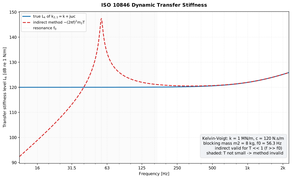
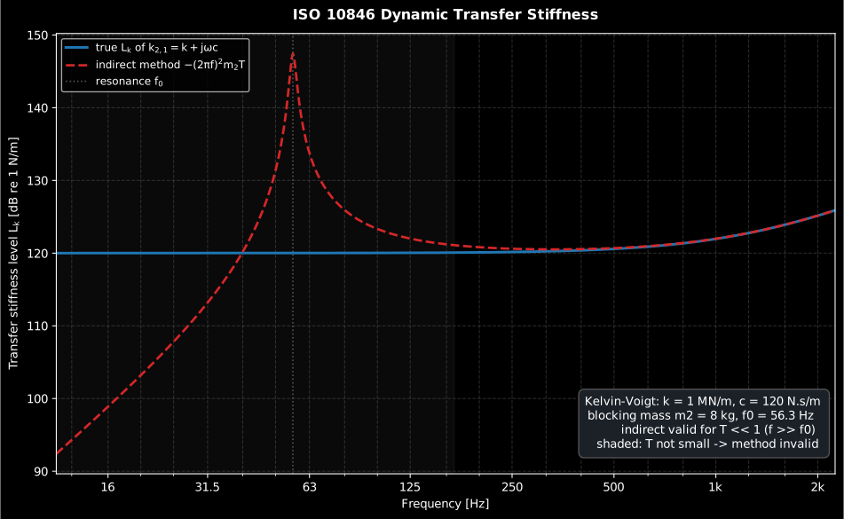
• Impedance mismatch (Inequality 2). Valid only where $\Delta L_{1,2}=L_{a1}-L_{a2}\ge 20\text{dB}$, i.e. $|T|\le 0.1$, the constant TRANSMISSIBILITY_LIMIT. transfer_stiffness_indirect computes $|T|$ at every frequency line and emits a TransferStiffnessWarning when any line exceeds it (routine near or below the mass/spring resonance, as in the figure above); the result it builds marks those lines as not valid, and its band average leaves them out.
• Rigid blocking mass (Inequality 3). Above an upper frequency $f_3$ the blocking mass no longer moves as a rigid body; results are valid only while its measured effective mass $m_{2,\text{eff}}=2F_2/(a_1^{\prime }+a_1^{\prime \prime })$ (Eq. 4) stays within 1 dB of the rigid mass: $|10{\log }_{10}(m_{2,\text{eff}}^2/m_2^2)|\le 1\text{dB}$. effective_blocking_mass finds $f_3$ from that measurement (section 5).
• Linearity (clause 7.6). Two input spectra 10 dB apart must give transfer-stiffness levels within 1.5 dB. The number is not arbitrary and it is the one criterion here that is really about the material: ISO 10846-1 Annex D collects the physics. Dynamic properties depend on preload, vibration amplitude, frequency and temperature; for filled rubber the in-phase modulus and the phase angle are essentially amplitude-independent below shear strain amplitudes of order $10^{-3}$ and fall significantly above about $2\times 10^{-3}$, the more so the higher the carbon-black content. So the elements that fail are the highly filled rubbers and anything with a designed amplitude dependence: a hydraulic mount is strongly amplitude-dependent by design, and cannot be described by a single $L_k$ spectrum at all. That makes the criterion actionable rather than pass/fail: the strain amplitudes occurring in service dictate the test amplitudes, and clause 7.6 says what the result then means, namely that the data may only be claimed valid for input amplitudes equal to or lower than the higher of the two tested. The upper bound of validated input level goes in the test report.

Every criterion above is a property of the element and the model. ISO 10846-2 clauses 6 and 7 add a set of pre-runs and hardware requirements that decide whether a result exists at all. One of the two level differences, the unidirectionality pre-run, can be judged from the measured spectra (check_unwanted_input, section 5); the background pre-run and the rest are left to the operator.

• A background pre-run (7.6.1). With the source switched off, measure $L_{F_2}$ and $L_{a_1}$; the source output shall be adjusted so that they exceed the background by at least 15 dB in every band of interest.
• A unidirectionality pre-run (6.4, Inequality 3). The acceleration in the excitation direction shall exceed the unwanted perpendicular components by at least 15 dB, measured at the edge of the excitation mass in the plane of the input flange: the accelerometer drawn on the rig figure. Bands that fail are excluded from the result; check_unwanted_input judges them. (Clause 7.6.1 sends this exclusion to “6.1, Inequality (1)”, the 20 dB of the blocked output; the condition it means is 6.4, Inequality (3), as the companion parts show. See the errata.)
• Transducers (6.5, 6.6). Accelerometers and force transducers shall have a sensitivity level that is frequency-independent within 0,5 dB, be calibrated at the laboratory temperature, and have a cross-axis sensitivity below 5 %. Where several transducer signals are summed, the resultant sensitivity function shall meet the same 0,5 dB requirement.
• Analyser (6.8). The spectral resolution shall give at least five distinct frequencies in every one-third-octave band of interest, and the frequency-response difference between the input-acceleration and output-force channels shall be under 0,5 dB or else applied as a correction.
• Coherence between the input and output signals is the recommended running indicator (7.6.2): it flags poor signal-to-noise and non-linearity, and it is read exactly as the mobility guide’s Annex A.1 list reads it.

Annex B of Part 2 says what each of these is worth. Its uncertainty budget assigns 0,3 dB to signal processing and background noise, 0,5 dB to instrumentation when only the minimum requirements above are met, 0,5 dB to the test rig (from the residual output motion the two inequalities bound), and 0,5 dB to linearity. The last two are rectangular terms over a 1,5 dB range, $1,5/(2\sqrt{3})=0,433$ dB each, which the annex rounds up to 0,5 dB. The three are comparable, which is the argument for not skipping any of them: no one of them dominates, so no one of them is optional.

import matplotlib.pyplot as plt
import numpy as np
from phonometry import vibration

# Kelvin-Voigt isolator k + jwc loaded by an 8 kg blocking mass.
k, c, m2 = 1.0e6, 120.0, 8.0
f0 = np.sqrt(k / m2) / (2.0 * np.pi)
f = np.logspace(np.log10(f0 / 5.0), np.log10(f0 * 40.0), 600)

k_true = k + 1j * 2.0 * np.pi * f * c
t = vibration.base_transmissibility(f, m2, k, c)
k_indirect = vibration.transfer_stiffness_indirect(f, t, m2)  # warns where T is not small

# One line: the indirect determination bundled as a result draws its own
# Lk(f) level spectrum:
res = vibration.indirect_transfer_stiffness_result(f, t, blocking_mass=m2)
res.plot()
plt.show()

# By hand, the true element stiffness against the indirect-method estimate:
fig, ax = plt.subplots()
ax.semilogx(f, vibration.transfer_stiffness_level(k_true),
            label="true $L_k$ of $k+j\\omega c$")
ax.semilogx(f, vibration.transfer_stiffness_level(k_indirect), "--",
            label="indirect method $-(2\\pi f)^2 m_2 T$")   # no flange here
ax.axvline(f0, color="0.6", linestyle=":", label="resonance $f_0$")
ax.set(xlabel="Frequency [Hz]", ylabel="Transfer stiffness level $L_k$ [dB re 1 N/m]")
ax.grid(True, which="both", alpha=0.3)
ax.legend()
plt.show()

The criterion, and the error it buys. The indirect method is valid from where $|T|$ falls below 0.1 (187.5 Hz for this element, not the mass/spring resonance at 56 Hz and not the $3f_0$ rule of thumb) and that limit is chosen because it is what holds the stiffness error inside the 1 dB the clause requires, as the middle panel’s second axis shows. The lower panel is the loss factor: for a Kelvin-Voigt element $\eta =\omega c/k$ rises in proportion to frequency, which is the model’s main deficiency as a description of real rubber, whose loss factor is far flatter. The definition holds only in the low-frequency range where inertial forces inside the element are negligible.

The blocking-force idealisation itself is quantified by ISO 10846-1, Eq. (6): for an isolator of output driving-point stiffness $k_{2,2}$ on a termination of stiffness $k_{\mathrm{t}}$, the delivered force is $F_2/F_{2,\mathrm{b}}=1/(1+k_{2,2}/k_{\mathrm{t}})$, within 10 % of the blocking force for $|k_{2,2}|<0.1|k_{\mathrm{t}}|$ (Eq. 7):

import warnings
from phonometry import vibration

# |T| = 0.5 violates Inequality (2): the indirect result is flagged.
with warnings.catch_warnings(record=True) as caught:
    warnings.simplefilter("always")
    vibration.transfer_stiffness_indirect(50.0, 0.5, blocking_mass=10.0)
print(caught[0].category.__name__)                     # TransferStiffnessWarning

# Blocking-force approximation at the 10 % limit (ISO 10846-1, Eq. 6):
print(round(abs(complex(vibration.blocking_force_ratio(1e5, 1e6))), 4))   # 0.9091

A swept or stepped measurement gives $k_{2,1}$ at hundreds of lines, and every part of the series reports it as one value per one-third-octave band: the squared magnitude averaged over the $n$ lines the band holds (ISO 10846-2 Formula (6), -3 Formula (7), -4 Formula (11), -5 Formula (6)),

“where the summation is performed over a minimum of $n=5$ frequencies”. Averaging the square rather than the level weights the peaks, which the parts call “usually the most important ones”, and the phase is lost. The five lines are also a requirement on the measurement: the analyser shall resolve at least five distinct frequencies per band, and a stepped or swept sine shall put five in every band for which a value is reported. So band_averaged_stiffness gives a band of one to four lines no value (NaN) and a TransferStiffnessWarning, rather than an average of too few lines. It assigns each line to the base-ten band that encloses it, names the bands by their ISO 266 centres, and leaves out first the lines that failed an adequacy condition, since every part excludes those from the evaluation: the indirect result marks the lines with $|T|>0.1$, so its .band_average() averages only the valid part of the sweep.

import warnings
import numpy as np
from phonometry import vibration

# Direct method, a Kelvin-Voigt mount k + jwc, lines every 2 Hz:
f = np.arange(90.0, 1120.0, 2.0)
k21 = 1.0e6 + 1j * 2.0 * np.pi * f * 80.0
direct = vibration.TransferStiffnessResult(
    frequencies=f, transfer_stiffness=vibration.transfer_stiffness_direct(k21 * 1e-6, 1e-6)
)
bands = direct.band_average()
print(bands.nominal_frequencies[[0, -1]], bands.line_counts[[0, -1]])  # [ 100. 1000.] [ 12 114]
print(round(float(bands.levels[-1]), 2))                               # 120.99  dB re 1 N/m

# Indirect method on an 8 kg blocking mass: |T| falls to 0.1 at 187.5 Hz, so the
# lines up to 186 Hz fail Inequality (2) and never reach the average; the 200 Hz
# band averages its 18 lines from 188 Hz up.
t = vibration.base_transmissibility(f, mass=8.0, stiffness=1.0e6, damping=120.0)
with warnings.catch_warnings():
    warnings.simplefilter("ignore", vibration.TransferStiffnessWarning)
    indirect = vibration.indirect_transfer_stiffness_result(f, t, blocking_mass=8.0)
bands = indirect.band_average()
print(bands.nominal_frequencies[0], bands.line_counts[0])  # 200.0 18
bands.plot()   # the band levels, the undetermined bands marked (needs matplotlib)

Three of the adequacy conditions of the series are level differences or a mass, and can be judged from what the rig measured. Each check returns the condition frequency by frequency with an overall .passes, draws itself with .plot(), and warns (TransferStiffnessWarning) where the condition fails.

• The output is blocked, $\Delta L_{1,2}=L_{a1}-L_{a2}\ge 20$ dB (ISO 10846-5 Inequality (1); Inequality (1) of Part 2, (2) of Parts 3 and 4): check_blocked_output. A smaller difference means too little stiffness mismatch between the element and the foundation, or flanking transmission.

• The input moves in one direction, the excitation direction at least 15 dB above each perpendicular one (Part 5 Inequality (2); (3) of Part 2, (5) of Part 3, (7) of Part 4): check_unwanted_input, which takes one row of levels per unwanted direction and lets the loudest decide.

• The mass in front of the output force transducers is light enough for the direct method (ISO 10846-4 Inequality (3), ISO 10846-2 Inequality (2)): the output flange, the force-distribution plate and half the transducers, $m_0$, carry an inertia force $m_0{a}_2$ the transducers read as part of the blocking force, and it shall not exceed 6 % of the force,

  $$m_0\le 0,06\times \frac{10^{L_{F2}/20}}{10^{L_{a2}/20}}\text{kg},$$

  with $L_{F2}$ re 1 µN and $L_{a2}$ re 1 µm/s², so the bound is $0,06|F_2|/|a_2|$. At the bound the force levels differ by $20\lg 1,06=0,51$ dB when the inertia force is in phase with the measured one and by $-20\lg 0,94=0,54$ dB when it opposes it: the 0,5 dB of NOTE 1 (which ISO 10846-4 prints as “05 dB”; see the errata). check_output_mass returns the limit and that worst-case bias, bias_bound_db.

For the indirect method the question is how high the blocking mass stays rigid. ISO 10846-4 Formula (6) (ISO 10846-3 Formula (4)) measures its effective mass with the block on soft springs, driven by a force $F_2$ through its centre of mass and read by two accelerometers $\sqrt{S}$ apart inside the contact area, $m_{2,\mathrm{eff}}=|2F_2/(a_1^{\prime }+a_1^{\prime \prime })|$; the upper limit $f_3$ is the lowest frequency at which it departs from $m_2$ by more than 1 dB (12 %), Inequality (5), with a departure below 40 Hz ignored as the mass-spring behaviour of the block on its supports. effective_blocking_mass interpolates the crossing between the last line inside the 1 dB and the first line outside it.

import numpy as np
from phonometry import vibration

f = [63.0, 125.0, 250.0]
check = vibration.check_blocked_output(f, [110.0, 110.0, 110.0], [85.0, 88.0, 86.0])
print(check.holds, check.passes)                        # [ True  True  True] True

# m0 = 0.4 kg (output flange, force distribution plate and half the transducers)
# under an output force of 1 N (120 dB re 1 µN) and an output acceleration of
# 0.1 m/s² (100 dB re 1 µm/s²):
mass = vibration.check_output_mass([125.0], 0.4, [120.0], [100.0])
print(mass.mass_limit_kg, mass.passes, mass.bias_bound_db.round(3))   # [0.6] True [0.355]

# A 20 kg block whose effective mass grows as (f/3 kHz)^2 above rigid:
fe = np.geomspace(20.0, 5000.0, 400)
m_eff = 20.0 * (1.0 + (fe / 3000.0) ** 2)
ones = np.ones(fe.size, dtype=complex)
block = vibration.effective_blocking_mass(fe, m_eff * ones, ones, ones, blocking_mass_kg=20.0)
print(round(block.upper_frequency_limit_hz, 1))         # 1047.9  Hz

With the output of the element blocked, the input force and the input acceleration give the driving-point stiffness (Formula (3)),

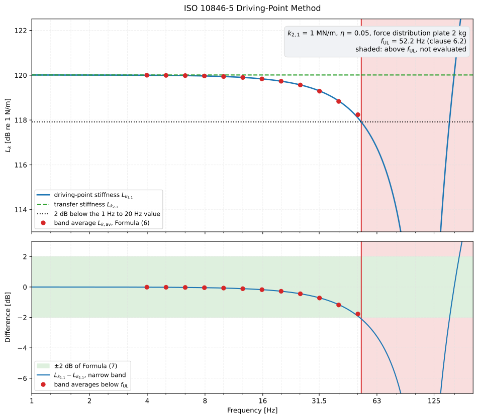
which equals the transfer stiffness only at low frequencies. Two things pull it away: the mass between the element and the input force transducers, whose inertia the transducers read with the element, and the element’s own internal resonances. Clause 6.2 fixes where the approximation ends. The low-frequency value is “the average for 1 Hz to 20 Hz”, and the upper limiting frequency $f_{\mathrm{UL}}$ is “the lowest frequency, at which the driving point stiffness level becomes 2 dB smaller than the low-frequency stiffness”. Up to it the band averages of $k_{1,1}$ stand for those of $k_{2,1}$ within 2 dB (Formula (7), $k_{\mathrm{av}}=k_{\mathrm{av}(2,1)}\approx k_{\mathrm{av}(1,1)}$), and above it the method has nothing to say. Typically $f_{\mathrm{UL}}$ lies between 50 Hz and 200 Hz, so this is a low-frequency method, meant for the owners of driving-point rigs.

driving_point_stiffness computes $k_{1,1}$, takes the low-frequency value as the Formula (6) average of the lines from 1 Hz to 20 Hz (for the flat stiffness the clause presumes, the same as the mean of the levels), and interpolates the crossing of the 2 dB threshold. Given the output acceleration or the unwanted input accelerations, it checks Inequalities (1) and (2) line by line and leaves the lines that fail out of everything, as 7.6.1 requires. Its .band_average() averages only the valid lines, those at or below $f_{\mathrm{UL}}$ (8.3 states the 2 dB “if $f\le f_{\mathrm{UL}}$”). For those bands the 2 dB of Formula (7) is the standard’s own statement, which Annex B assumes again for its budget (B.3.5): the criterion of 6.2 only watches $k_{1,1}$ fall below its own low-frequency value, so nothing in the average proves the bound line by line. Below 20 Hz, 7.5 asks for a 0,2 Hz line spacing rather than five lines per band, which leaves the lowest bands short of five; those bands have no value, without a warning, and the note to clause 9 m) accepts narrow-band data there instead.

import matplotlib.pyplot as plt
import numpy as np
from phonometry import vibration

# A 1 MN/m element with a 5 % loss factor, driven through a 2 kg force
# distribution plate: the input force transducers read the plate's inertia with
# the element.
f = np.arange(1.0, 200.0, 0.2)          # the 0.2 Hz lines of 7.5
w = 2.0 * np.pi * f
k21 = 1.0e6 * (1.0 + 0.05j)
res = vibration.driving_point_stiffness(f, (k21 - w**2 * 2.0) * 1e-6, -(w**2) * 1e-6)
print(round(res.upper_limiting_frequency_hz, 1))    # 52.2  Hz

# One line each: the level with the 2 dB threshold and f_UL, and the bands.
res.plot()
res.band_average().plot()
plt.show()

# By hand, the two panels above: k1,1 against k2,1, and their difference.
bands = res.band_average()
centres = bands.center_frequencies[bands.determined]
band_levels = bands.levels[bands.determined]
l21 = 20.0 * np.log10(abs(k21))
f_ul = res.upper_limiting_frequency_hz
fig, (top, bottom) = plt.subplots(2, 1, sharex=True, figsize=(10, 8.8))
for panel in (top, bottom):
    panel.axvspan(f_ul, f[-1], color="0.9")            # above f_UL: not evaluated
    panel.axvline(f_ul, color="C1")
    panel.grid(True, which="both", alpha=0.3)
top.semilogx(f, res.levels, label="driving-point stiffness $L_{k_{1,1}}$")
top.axhline(l21, color="C2", linestyle="--", label="transfer stiffness $L_{k_{2,1}}$")
top.axhline(res.threshold_level_db, color="k", linestyle=":",
            label="2 dB below the 1 Hz to 20 Hz value")
top.plot(centres, band_levels, "o", color="C1",
         label="band average $L_{k,\\mathrm{av}}$, Formula (6)")
top.set(ylabel="$L_k$ [dB re 1 N/m]", ylim=(l21 - 7.0, l21 + 2.5))
top.legend(loc="lower left")
bottom.axhspan(-2.0, 2.0, color="C2", alpha=0.15, label="$\\pm$2 dB of Formula (7)")
bottom.semilogx(f, res.levels - l21, label="$L_{k_{1,1}} - L_{k_{2,1}}$, narrow band")
bottom.plot(centres, band_levels - l21, "o", color="C1",
            label="band averages below $f_\\mathrm{UL}$")
bottom.set(xlabel="Frequency [Hz]", ylabel="Difference [dB]",
           xlim=(f[0], f[-1]), ylim=(-7.0, 3.0))
bottom.legend(loc="lower left")
plt.show()

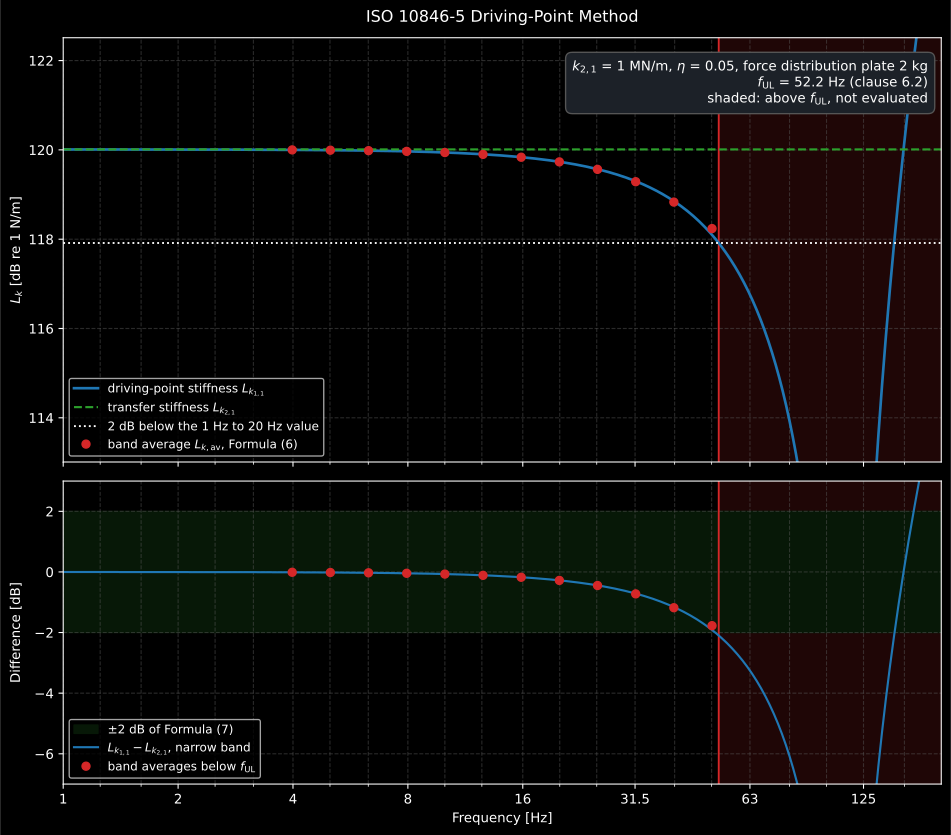
Where the method stops. The force distribution plate between the input force transducers and the element is 2 kg, $m_{\mathrm{p}}$, so the measured stiffness is $k_{2,1}-{\omega }^2{m}_{\mathrm{p}}$ and falls away from the transfer stiffness as the frequency rises; at 52.2 Hz it is 2 dB below its 1 Hz to 20 Hz value, and nothing above that is evaluated. Every band average below it lies inside the ±2 dB of Formula (7); the last one, at 50 Hz, averages only the 37 lines below $f_{\mathrm{UL}}$ and sits 1.8 dB down.

The uncertainty budget (Annex B) writes the band level as the measured one plus five corrections of zero estimate, each with sensitivity coefficient 1 (Formula (B.1)), combines them by root sum of squares (B.2) and takes $U=2u$ for 95 % coverage (B.3). driving_point_uncertainty builds it on metrology.combine_uncertainty: signal processing 0,3 dB and instrumentation 0,5 dB (normal), installation repeatability $p/\sqrt{3}$ for a spread $2p$ of repeated installations, and three rectangular terms, the test rig $1/(2\sqrt{3})=0,289$ dB, the driving-point discrepancy $2/\sqrt{3}=1,155$ dB for its $\pm 2$ dB, and linearity $1,5/(2\sqrt{3})=0,433$ dB. Those three are the expressions the annex prints. Table B.1 carries them rounded up to one decimal, 0,3, 1,2 and 0,5 dB, the conservative rounding an uncertainty may take (ISO/IEC Guide 98-3, 7.2.6), which puts $u$ at 1,456 dB instead of 1,394 dB with no repeatability spread. The library keeps the expressions, and every term can be passed in to reproduce the table or to state a reasoned estimate. The discrepancy term dominates: it is the price of measuring $k_{1,1}$ for $k_{2,1}$.

from phonometry import vibration

budget = vibration.driving_point_uncertainty(119.3, repeatability_range_db=0.6)
print(round(budget.combined_uncertainty_db, 3))    # 1.405  dB
print(round(budget.expanded_uncertainty_db, 2))    # 2.81  dB (U = 2u)
budget.plot()   # one bar per input quantity, with u and U

A level in dB re 1 N/m needs a scale before it means anything. Each decade of stiffness is 20 dB, so the working range spans roughly:

| Element | $|k_{2,1}|$ | $L_k$ | |---|---|---| | a soft rubber mount or a steel coil spring | $10^5$ N/m | 100 dB | | a general-purpose machine mount | $10^6$ N/m | 120 dB | | a stiff bonded pad or a hard elastomer | $10^7$ N/m | 140 dB | | a rigid connection (for comparison) | $10^8$ N/m and up | 160 dB and up |

Lower is better, and the shape matters more than the value: in the figure above the level rises with frequency, which is the isolator getting stiffer, and therefore less effective, exactly in the range where structure-borne noise matters. That rise is the single most useful thing an $L_k(f)$ spectrum tells an engineer about a mount, and it is what a datasheet quoting one static stiffness cannot say.

On its own $k_{2,1}$ still predicts nothing, because the blocked force is only what the element delivers to a receiver much stiffer than itself. blocking_force_ratio prices that assumption against a real termination:

# The same 1 MN/m mount under a concrete floor and under a light timber one.
for k_t in (3e9, 2e6, 5e5):
    ratio = abs(complex(vibration.blocking_force_ratio(1e6, k_t)))
    print(f"{k_t:.0e}", round(ratio, 3))     # 1.0 / 0.667 / 0.333

On the concrete floor ($k_{\mathrm{t}}=3$ GN/m) the delivered force is the blocked force, Equation (7) is satisfied by three orders of magnitude, and the datasheet number is directly usable. On a lightweight floor of 2 MN/m it is not: only two thirds of the blocked force arrives (−3.5 dB), Equation (7) fails, and the mount’s characterisation no longer predicts what the installation does. That is not the isolator failing (a mobile receiver takes less force, so the real installation is quieter than the blocked-force estimate); it is the single-number description failing, and the route out is a prediction that carries both mobilities: installed structure-borne sound (EN 12354-5), fed by a source characterised through EN 15657. The rule behind both is the source/receiver mobility rule of the mobility guide.

The dynamic stiffness is a member of the frequency-response-function family (ISO 10846-1, Annex A / Table A.2): it is the reciprocal of the receptance and relates to the mechanical impedance $Z$ and effective mass $m_{\text{eff}}$ by $k=j\omega Z=-{\omega }^2{m}_{\text{eff}}$. These conversions are the same as the mechanical mobility convert_frf pivot:

from phonometry import vibration

k = 1e6 + 5e4j                                  # N/m, at 250 Hz
Z = vibration.convert_frf(k, 250.0, "dynamic_stiffness", "impedance")
print(round(abs(complex(vibration.convert_frf(
    Z, 250.0, "impedance", "dynamic_stiffness"))), 1))    # 1001249.2

TransferStiffnessResult.report(path) renders a one-page dynamic-transfer-stiffness characterisation report for a resilient element (ISO 10846-1:2008 definition; determined by the direct method, ISO 10846-2:2008, or the indirect blocking-mass method, ISO 10846-3:2002). The sheet shows the $L_k(f)$ level spectrum beside a compact table of characteristic points (the determination method, the blocking mass for the indirect method, the frequency range, and the low-frequency stiffness plateau $|k_{2,1}|$, its level $L_k$ and the loss factor there), then the one-third-octave band levels $L_{k,\mathrm{av}}$ of section 4, which the test report of both parts presents (ISO 10846-2 9 m), ISO 10846-3 10 j)), and a boxed low-frequency $L_k$ (the plateau that characterises the element below its internal resonances). The characteristic points are read at the lowest valid line and the spectrum draws the excluded lines apart, so an indirect result never reports the resonance region that Inequality (2) rules out; a band of fewer than five valid lines prints its line count instead of a level. It is a characterisation, so there is no pass/fail verdict; language="es" renders the Spanish fiche. The fiche always embeds the $L_k(f)$ spectrum, so it needs both the report and plot extras (pip install "phonometry[report,plot]").

import numpy as np
from phonometry import ReportMetadata, vibration

# Ten lines in every one-third-octave band from 20 Hz to 2 kHz:
freqs = 1000.0 * 10.0 ** ((np.arange(-175, 35) + 0.5) / 100.0)
k21 = 1e6 + 1j * (2 * np.pi * freqs) * 80.0     # Kelvin-Voigt element k + jwc
u1 = 1e-6 + 0j
k = vibration.transfer_stiffness_direct(k21 * u1, u1)     # direct method: k2,1 = F2,b/u1
res = vibration.TransferStiffnessResult(frequencies=freqs, transfer_stiffness=k)
res.report(
    "transfer_stiffness.pdf",
    metadata=ReportMetadata(
        specimen="Rubber vibration isolator",
        measurement_standard="ISO 10846-2",
    ),
)   # one-page fiche (needs phonometry[report,plot])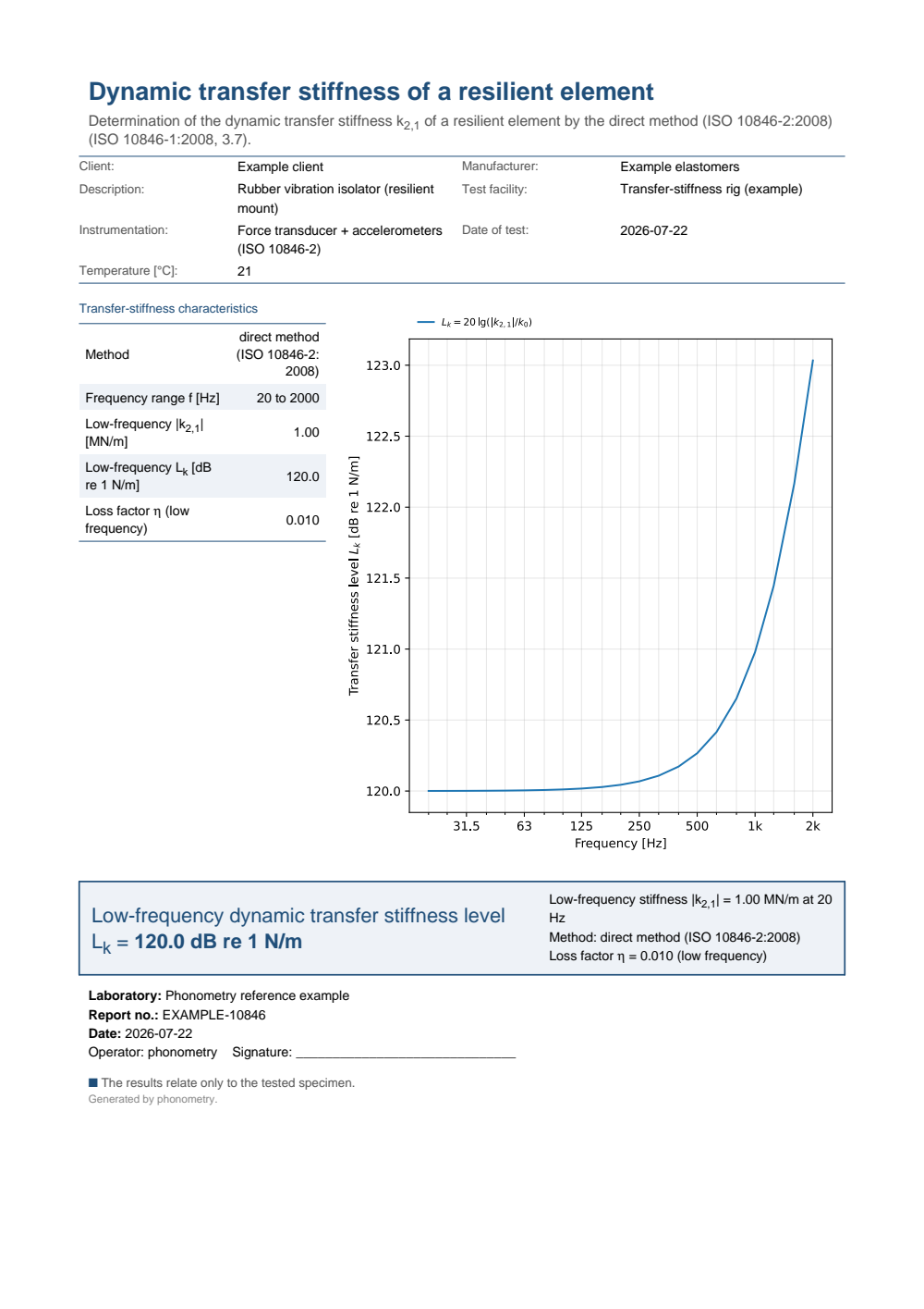

One-page dynamic-transfer-stiffness fiche: a metadata header, a table of the FRF characteristic points (the determination method, the frequency range and the low-frequency stiffness, level and loss factor) beside the transfer-stiffness level spectrum, the 21 one-third-octave band levels from 20 Hz to 2 kHz, and the boxed low-frequency level.

Download the report (PDF)

• Covered

  ISO 10846-1:2008’s $k_{2,1}=F_{2,\mathrm{b}}/u_1$ definition, the level (ISO 10846-2 and -3, 3.17) and loss factor (ISO 10846-1, 3.8) (transfer_stiffness_level, loss_factor), the ISO 10846-2:2008 direct method (transfer_stiffness_direct), and the ISO 10846-3:2002 indirect method of Formula 1 (transfer_stiffness_indirect, including its flange_mass= term). The blocking-force approximation of Equations 6-7 (blocking_force_ratio) and the Annex A / Table A.2 FRF relations (convert_frf) are implemented too. TransferStiffnessResult bundles a swept determination, and .report() renders the characterisation fiche with its one-third-octave band levels.

• Covered

  The one-third-octave band average of every part, ISO 10846-2 Formula (6), -3 Formula (7), -4:2003 Formula (11) and -5:2008 Formula (6), with no value for a band of fewer than five lines (band_averaged_stiffness, TransferStiffnessResult.band_average). The adequacy conditions ISO 10846-4:2003 and -5:2008 state as inequalities: the 20 dB of the blocked output and the 15 dB of the unwanted input directions (check_blocked_output, check_unwanted_input) and the output-mass limit of ISO 10846-4 Inequality (3) (check_output_mass), and the effective blocking mass of ISO 10846-4 Formula (6) with its $f_3$ (effective_blocking_mass). The ISO 10846-5:2008 driving-point stiffness of Formula (3), its upper limiting frequency (6.2) and the band averages of Formula (7) (driving_point_stiffness), and the Annex B uncertainty budget (driving_point_uncertainty). Neither part prints a worked example, so conformance is anchored on closed forms.

• Not covered

  The test arrangements of ISO 10846-4 for couplings, bellows, hoses, pipe hangers and cables are described by the standard, not modelled: the same functions serve them once the forces and accelerations are measured. The Figure 11 nomograms of $f_3$ for steel cubes and cylinders are not tabulated; $f_3$ is found from a measured effective mass. The linearity test (two input spectra 10 dB apart within 1.5 dB, clause 7.7 of ISO 10846-2, -4 and -5 and clause 7.6 of ISO 10846-3) is not checked in code, and neither are the preload, creep and temperature conditioning, the background pre-run, the 0,5 dB transducer flatness and inter-channel matching or the 0,2 Hz line spacing ISO 10846-5 asks for below 20 Hz: the page describes them and leaves them to the operator. Hydraulic mounts are outside the single-spectrum description altogether: their stiffness is amplitude-dependent by design, so one $L_k(f)$ does not characterise them.

References

Section titled “References”- Cremer, L., Heckl, M., & Petersson, B. A. T. (2005). Structure-borne sound: Structural vibrations and sound radiation at audio frequencies (3rd ed.). Springer. https://doi.org/10.1007/b137728Vibration isolation theory: why an isolator's performance depends on the source and receiver mobilities, the physics behind the blocked-force characterisation. ISBN 978-3-540-22696-3.
- International Organization for Standardization. (2002). Acoustics and vibration — Laboratory measurement of vibro-acoustic transfer properties of resilient elements — Part 3: Indirect method for determination of the dynamic stiffness of resilient supports for translatory motion (ISO 10846-3:2002). The indirect method k₂₁ = −(2πf)²(m₂+m_f)T (Formula 1) with its validity conditions (clause 6: Inequalities 2 and 3; clause 7.6 linearity). Conformance is anchored on the indirect inertia relation, the |T| = 0.1 ↔ ΔL₁,₂ = 20 dB validity limit and its 1 dB (12 %) accuracy bound, and the 7.6 linearity criterion.
- International Organization for Standardization. (2003). Acoustics and vibration — Laboratory measurement of vibro-acoustic transfer properties of resilient elements — Part 4: Dynamic stiffness of elements other than resilient supports for translatory motion (ISO 10846-4:2003). Couplings, bellows, hoses, pipe hangers and cables by the direct and the indirect method: the output-mass limit of Inequality (3), the effective blocking mass of Formula (6) with its f₃ (Inequality 5), and the band average of Formula (11). It prints no worked example, so conformance is anchored on closed forms; the 0,5 dB of its 6.2 NOTE 1 is printed as 05 dB (see the errata).
- International Organization for Standardization. (2008). Acoustics and vibration — Laboratory measurement of vibro-acoustic transfer properties of resilient elements — Part 1: Principles and guidelines (ISO 10846-1:2008). The principles part of the series: the blocking-force idealisation and the FRF relations this page implements: the dynamic transfer stiffness k₂₁ = F₂,b/u₁ and its FRF relations (clause 5 and Annex A / Table A.2) and the blocking-force approximation (Eqs. 6/7). Parts 4 and 5 of the series extend the same quantities to elements other than supports and to the driving-point low-frequency method. Conformance is anchored on the closed-form Table-A.2 identity k = jω·Z and the Eq. (6) force ratio 1/1.1.
- International Organization for Standardization. (2008). Acoustics and vibration — Laboratory measurement of vibro-acoustic transfer properties of resilient elements — Part 2: Direct method for determination of the dynamic stiffness of resilient supports for translatory motion (ISO 10846-2:2008). The direct method, and (with Part 3) the level L_k re 1 N/m and the loss factor (clauses 3.8/3.17). Conformance is anchored on the closed-form level of a decade of stiffness.
- International Organization for Standardization. (2008). Acoustics and vibration — Laboratory measurement of vibro-acoustic transfer properties of resilient elements — Part 5: Driving point method for determination of the low-frequency transfer stiffness of resilient supports for translatory motion (ISO 10846-5:2008). The driving-point stiffness k₁,₁ of Formula (3), the upper limiting frequency of 6.2, the band averages of Formulas (6) and (7), Inequalities (1) and (2), and the Annex B budget. No worked example either; Table B.1 rounds its three rectangular terms up to one decimal (the linearity term 1,5/(2√3) = 0,433 dB becomes 0,5 dB), and the library keeps the expressions.