Verifying a human-vibration meter
Standards: ISO 8041Key references: Griffin 1996
Every other page in this section computes something about a vibration a person is exposed to: what a day of it does to the body, what repeated shocks do to the spine, what a seat passes on. This one computes something about the instrument. ISO 8041-1 is not a method for measuring vibration; it is the specification a general-purpose human-vibration meter is designed and tested against, and the rest of the section has been quoting one clause of it all along, because the nine frequency weightings that human vibration exposure applies are defined here and nowhere else.
The human in that name is load-bearing. The standard specifies instruments “designed to measure vibration values, for the purpose of assessing human response to vibration” (clause 1), for hand-transmitted vibration (ISO 5349-1), whole-body vibration (ISO 2631-1, ISO 2631-2 and ISO 2631-4) and low-frequency whole-body vibration from 0,1 Hz to 0,5 Hz. General purpose separates it from ISO 8041-2, which specifies personal vibration exposure meters with most of the same tables (section 11 says which), and not from some other kind of vibration meter: an instrument for machine condition monitoring or for damage to buildings is graded against other documents, and nothing on this page applies to it.
The clause that comes right after those definitions is where this page starts: how far a real instrument may sit from those weightings before it stops conforming. That one is a table of frequencies and percentages, and a subtraction. It turns out not to be alone. The characteristic phase deviation, the running r.m.s. decay and the saw-tooth signal burst are all specified as numbers a conforming meter has to produce, and every one of those numbers can be computed. This page is about the parts of a type test that are arithmetic rather than laboratory work, and about being clear on where each of them stops.
1. Why an instrument standard is in a library of computations
Section titled “1. Why an instrument standard is in a library of computations”ISO 8041-1 defines three levels of performance testing (clause 1): pattern evaluation, a full test of the instrument against every specification in the document, with validation as its reduced form for a one-off instrument; periodic verification, an intermediate set of tests that confirms an instrument still performs as specified; and in situ checks, the minimum that indicates it is likely to be working. All three are work on hardware, done in a laboratory or in the field. None of them is run here.
What recurs inside all three is a single calculation. Somebody measured the
frequency response of a weighting channel; the standard prints the response it
should have had and the band it is allowed to sit in; does the measurement
fall inside the band? No shaker, no reference transducer and no climate
chamber are needed to answer that, only the design goal and two tables. That
is what verify_weighting does, and it is all it does.
So the scope of this page is narrow and worth stating before anything else. What the library holds is the arithmetic: the design goal (the exact transfer functions of clause 5.6, already used to weight signals elsewhere in this section), the transition frequencies of Table 4 and the tolerance bands of Table 5, the reference conditions of Table 1 and the tolerances of indication of Table 2, the characteristic phase deviation of Formula (6), the running r.m.s. decay times of Tables 10 and 11, and the 228 signal-burst indications of Tables 7 to 9. Every one of those is either a number the standard prints or a number it defines in closed form, and every one of them is one side of a comparison whose other side comes from a bench.
What the library does not hold is the bench. The accuracy of indication under reference conditions (5.5), amplitude linearity (5.7), instrument noise (5.8), overload and under-range indication (5.10 and 5.11), electrical cross-talk (5.16), the mounting of clause 6 and the environmental and electromagnetic criteria of clause 7 are measurements on hardware, and none of them is here. What is here is one half of each of the other comparisons: the standard’s own side of them, arithmetic that runs without a bench. The other half always needs one, because somebody has to shake a transducer and read a display. Passing the weighting check is a necessary condition for conformity and never a certificate of it.
One sentence of 5.6.6 is worth carrying through the rest of the page: the tolerance limits include the applicable maximum expanded uncertainties of measurement. The band is not the instrument’s allowance with the uncertainty of the bench measurement added on top; that uncertainty has to fit inside the band as well. There is a second sentence about uncertainty, in 13.1 and 14.1, and it says something different; section 4 is about telling the two apart.
How the measurement goes
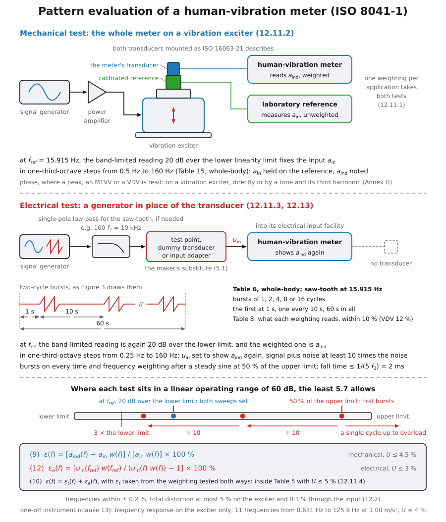
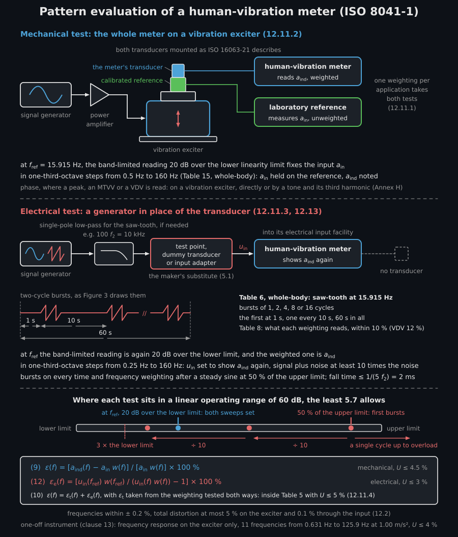
Section titled “How the measurement goes”In a pattern evaluation (clause 12), submit the meter with its transducer, mounting, cable and input adaptors, its sensitivity set by its documented procedure, and use traceably calibrated bench instruments with every test frequency within ±0.2 %. At the reference frequency, take at least three readings against a calibrated reference transducer at the same point: no more than 3 % apart, their mean inside Table 2.
Per application, one weighting goes through both tests and the others through either, a third of an octave apart at most over Table 15. On the exciter, with both transducers mounted as ISO 16063-21 describes, set the band-limited reading 20 dB above the lower linearity limit at the reference frequency, then hold that input on the reference transducer and note the reading at every frequency: Formula (9), within 4.5 % expanded uncertainty. Through the electrical input, hold the reading and note the input signal value, with signal plus noise at least ten times the noise: Formula (12), within 3 %. The transducer error of the weighting tested both ways completes the others, graded against Table 5 within 5 %. For the bursts, set a steady sine to 50 % of the upper linearity limit, apply the Table 6 saw-tooth to every weighting, and repeat tenfold lower down to three times the lower limit. A meter reading a peak, an MTVV or a VDV also has its phase checked by Annex H; a one-off instrument is shaken at the fixed frequencies of 13.10. Report every configuration, condition, result and actual uncertainty, and whether the meter conforms. A periodic verification (clause 14) is a different bench: it keeps only the mechanical sensitivity, linearity and frequency-response checks, for a whole-body meter at 1.995, 7.943, 15.85 and 63.10 Hz at 1.00 m/s² with U at most 5 %.
2. The nine weightings, and the band that widens around them
Section titled “2. The nine weightings, and the band that widens around them”The design goal is not a table of numbers, it is a transfer function. Clause
5.6 builds every weighting from four analog stages, a second-order Butterworth
high-pass and low-pass pair that band-limits, an acceleration-velocity
transition carrying the overall gain and an upward step, multiplied together
as
(Formula (5)). Human vibration covers that cascade and
the Table 3 parameter set that specialises it into the nine weightings Wb,
Wc, Wd, We, Wf, Wh, Wj, Wk and Wm. weighting_factors
evaluates it at any frequency, and that value, not a tabulated one, is what a
measurement is compared against. Annex B does tabulate the same weightings to
four significant figures, and says of itself that the values were calculated
from the design goals rather than defining them.
Around the design goal sits Table 5, and it is easy to read as one tolerance when it is three. The rows are keyed to four transition frequencies to that Table 4 gives per weighting, which cut the axis into five regions; the five printed rows carry only three distinct pairs of limits, because the two skirts share theirs and so do the two tails:
| Frequency region | Magnitude tolerance | Characteristic phase deviation |
|---|---|---|
| +26 %, −100 % | ±∞ | |
| +26 %, −21 % | ±12° | |
| +12 %, −11 % | ±6° | |
| +26 %, −21 % | ±12° | |
| +26 %, −100 % | ±∞ |
Note which rows are closed. The central region includes both of its corners, the skirts exclude theirs, so a measurement exactly at or takes the tighter limit rather than the wider one on the other side of it.
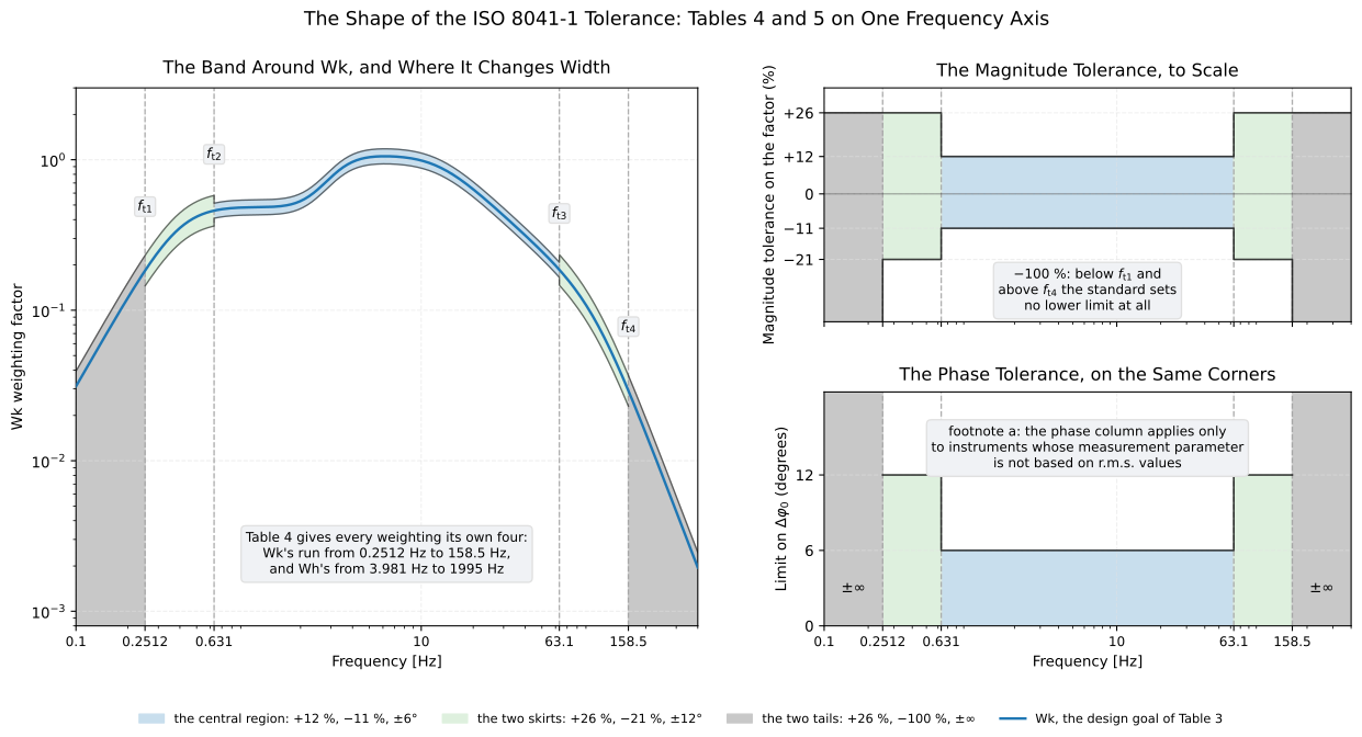
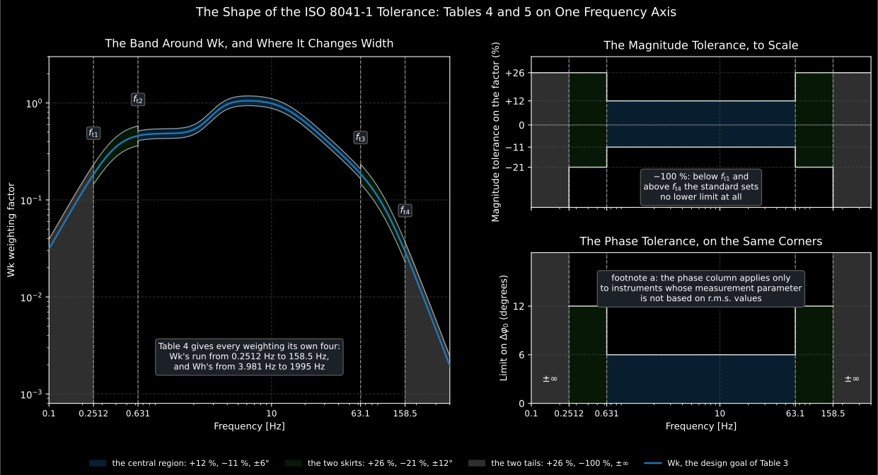
Table 4 prints each corner twice, as a power and as a rounded
decimal beside it, and the library builds them from the exponents. So
for Wk is 63.0957 Hz and the 63.1 Hz printed beside it is
the courtesy, not the value:
from phonometry import vibration
# Table 4 for Wk: ft1, ft2, ft3, ft4.print([round(f, 4) for f in vibration.TRANSITION_FREQUENCIES_HZ["Wk"]])# [0.2512, 0.631, 63.0957, 158.4893]
# Table 5 read across them: tail, skirt, central, skirt, tail.upper, lower = vibration.weighting_tolerance_percent(    "Wk", [0.2, 0.5, 16.0, 100.0, 200.0])print(upper)   # [26. 26. 12. 26. 26.]print(lower)   # [-100.  -21.  -11.  -21. -100.]
The one-third-octave centres are exact powers too, Hz (Formula (B.1)), which is what makes the corners land on band centres rather than beside them. Band 18 is Hz and is the last band of the central region, exactly as the Annex B tolerance column shows it; the same measurement entered as the printed 63.1 Hz falls a few thousandths of a hertz above and is graded against the skirt instead. Annex B says the same thing about the weighting factors: use the actual centre frequencies, never the nominal band labels.
print(vibration.weighting_tolerance_percent("Wk", [10 ** 1.8, 63.1])[1])# [-11. -21.]Where the corners sit. Table 1 also gives a nominal frequency range per application, and the Table 4 corners straddle it rather than coincide with it. Whole-body vibration is specified from 0.5 Hz to 80 Hz while the tight region runs from 0.631 Hz to 63.1 Hz; hand-transmitted vibration from 8 Hz to 1 000 Hz against 10 Hz to 794.3 Hz; low-frequency whole-body vibration from 0.1 Hz to 0.5 Hz against 0.1259 Hz to 0.3981 Hz. In all three cases both ends of the working range fall in a skirt, and the tails begin beyond it.
Why the band widens away from the middle. The percentages grow outwards, and the allowance they represent does not. A percentage says nothing about how much error it lets through until it is multiplied by the factor it is a percentage of. At the upper corner the design factor has already fallen by more than a decade, and at the lower one to a fifth of its peak:
from phonometry import vibration
ft1, ft2, ft3, ft4 = vibration.TRANSITION_FREQUENCIES_HZ["Wk"]corners = [ft1, ft2, 6.31, ft3, ft4]design = vibration.weighting_factors("Wk", corners)upper, _ = vibration.weighting_tolerance_percent("Wk", corners)
print(design.round(4))                   # [0.1832 0.4588 1.0544 0.1857 0.0292]print((design * upper / 100).round(4))   # [0.0476 0.0551 0.1265 0.0223 0.0076]
At 6.31 Hz the tight +12 % is worth 0.1265 in factor units; at 158.5 Hz the generous +26 % is worth 0.0076, about seventeen times smaller. The reading behind that, which the standard does not spell out, is the shape of the response: outside the working range the weighting is on a steep band-limiting roll-off, where a small error in a corner frequency turns into a large percentage error in the factor, while the same band contributes almost nothing to a weighted r.m.s. value. Where the contribution is large, in the middle, the standard is strict.
Judging a measured response. verify_weighting takes the frequencies a
response was measured at and the factors read there, evaluates the design goal
at the same frequencies and applies the acceptance test the tolerance columns
are written in, against the
band of the region each frequency falls in:
import numpy as npfrom phonometry import vibration
# A bench sweep of the Wk channel of a whole-body meter. The centres are# built from Formula (B.1) rather than typed as decimals: 63.096 rounds up# past ft3 and would be graded against the skirt, as the paragraph above# warns.bands = np.array([-3, 0, 3, 6, 9, 12, 15, 18, 19])frequencies = 10.0 ** (bands / 10.0)measured = np.array([0.4314, 0.4969, 0.5466, 0.9937, 1.068,                     0.7897, 0.3427, 0.1894, 0.1366])
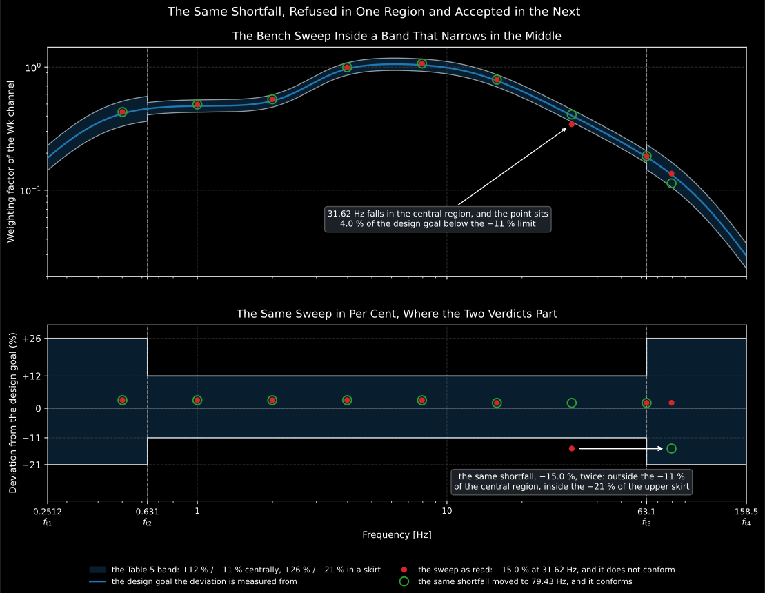
check = vibration.verify_weighting("Wk", frequencies, measured)print(check.passes)                             # Falseprint(check.deviation_percent.round(1))# [  3.   3.   3.   3.   3.   2. -15.   2.   2.]print(check.failing_frequencies_hz.round(2))    # [31.62]print(round(check.worst_deviation_percent, 1))  # -15.0
check.plot()   # the measurement inside its band (needs matplotlib)
A channel reading 2 % to 3 % high across the range passes, because that is inside +12 % and inside +26 %. The one band reading 15 % low fails, and it fails because of where it sits: 31.62 Hz is in the central region, whose lower limit is −11 %. Move the same shortfall to 79.43 Hz, which is between and , and the instrument conforms:
moved = np.array([0.4314, 0.4969, 0.5466, 0.9937, 1.068, 0.7897, 0.4112, 0.1894, 0.1138])print(vibration.verify_weighting("Wk", frequencies, moved).passes) # True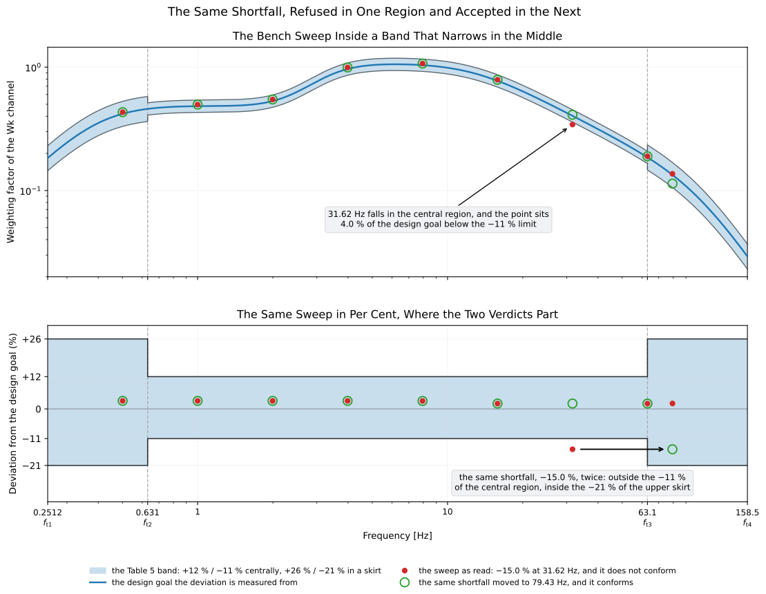
Show the code for the one-sweep tolerance-band view
import matplotlib.pyplot as pltimport numpy as npfrom phonometry import vibration
check = vibration.verify_weighting("Wk", frequencies, measured)
# One line:check.plot()plt.show()
# By hand, from the result's fields, mirroring what# WeightingVerification.plot() draws:upper, lower = vibration.weighting_tolerance_percent(    check.weighting, check.frequencies_hz)inside = check.within_tolerancefig, ax = plt.subplots()ax.fill_between(check.frequencies_hz,                check.design * (1.0 + lower / 100.0),                check.design * (1.0 + upper / 100.0),                color="#1f77b4", alpha=0.15, label="ISO 8041-1 tolerance")ax.plot(check.frequencies_hz, check.design, color="#1f77b4", lw=2.0,        label="design goal")ax.plot(check.frequencies_hz[inside], check.measured[inside], "o",        color="#2ca02c", label="within tolerance")ax.plot(check.frequencies_hz[~inside], check.measured[~inside], "X",        color="#d62728", markersize=9, label="outside tolerance")ax.set(xscale="log", yscale="log", xlabel="Frequency [Hz]",       ylabel="Weighting factor")ax.grid(True, which="both", alpha=0.3)ax.legend()plt.show()
3. −100 % is the absence of a lower limit, not a wide one
Section titled “3. −100 % is the absence of a lower limit, not a wide one”The most misreadable cell of Table 5 is the −100 % in its first and last
rows. It looks like an extremely generous tolerance. It is not a tolerance at
all: a factor 100 % below the design goal is zero, and no weighting factor can
be negative, so that limit admits every response there is. Below
and above the standard constrains the response
from above and stops constraining it from below altogether. An instrument may
roll off as steeply as its designer likes outside the working range, and one
that reads nothing at all out there conforms:
from phonometry import vibration
# The design goal at 0.1259 Hz, below ft1 = 0.2512 Hz for Wk.print(vibration.weighting_factors("Wk", [0.1259]).round(5))   # [0.04932]
# A channel that reads nothing at all there still conforms.dead = vibration.verify_weighting("Wk", [0.1259], [0.0])print(dead.passes, dead.deviation_percent.round(1))   # True [-100.]
# The upper limit is the half of the cell that can fail: +26 %, tail or not.high = vibration.verify_weighting("Wk", [0.1259], [0.0626])print(high.passes, high.deviation_percent.round(1))   # False [26.9]
Keep the asymmetry in view, because it is the point of those two rows. What
the standard is preventing out there is a meter that responds to vibration
it should be ignoring, never a meter that ignores it too well. The value is
published as UNCONSTRAINED_BELOW so a report can name it instead of writing
a bare number, and the verification compares against it as an ordinary limit:
the tail rows need no special case, since every non-negative factor satisfies
them by construction.
4. The laboratory’s uncertainty moves the measurement, not the band
Section titled “4. The laboratory’s uncertainty moves the measurement, not the band”Two sentences of the standard talk about expanded uncertainty and it is easy to read them as one. They are not, and a verdict computed with the wrong one of them is wrong in the direction that lets an instrument through.
The first is the sentence of 5.6.6 quoted at the end of section 1: the
tolerance limits of Table 5 include the applicable maximum expanded
uncertainties of measurement. That is a statement about how the table was
drawn. It is why weighting_tolerance_percent returns +12 % and −11 % and
never anything wider: the allowance for a careful bench is already inside
those numbers, and adding to them would spend it twice.
The second is in 13.1 and 14.1, word for word in both: compliance is
demonstrated when the measured deviation from a design goal, extended by the
actual expanded uncertainty of measurement of the testing laboratory, does
not exceed the specified tolerance limits. That is a statement about one
laboratory on one day. It moves the deviation, not the band, so the comparison
becomes deviation + U <= upper and deviation - U >= lower, and the number
U is the laboratory’s own, calculated with the coverage factor k = 2 that
both clauses print.
The two are consistent because they are about different numbers. 12.1 bounds
the laboratory’s U: a testing laboratory may not perform a test at all if
its actual expanded uncertainty exceeds the maximum the clause permits, and it
is those maxima that 5.6.6 says are already inside the printed limits. The
library publishes both sides, keyed by clause number, so a report can name the
figure it used:
from phonometry import vibration
# The most 12.11.2 lets a laboratory carry into a mechanical# frequency-response test, and the coverage factor it is expanded with.print(vibration.MAX_EXPANDED_UNCERTAINTY_PERCENT["12.11.2"])   # 4.5print(vibration.ISO8041_COVERAGE_FACTOR)                       # 2.0
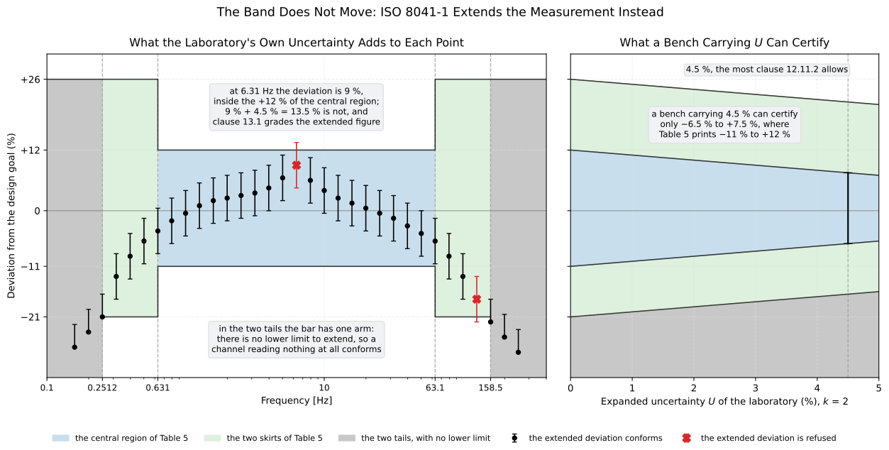
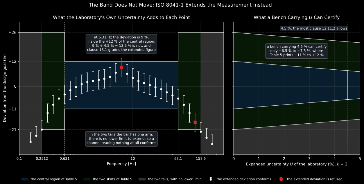
Here is what the difference does to a verdict. One band of a Wk sweep reads
9 % above the design goal at 6.31 Hz, which is inside the +12 % of the central
region with three points to spare:
frequency = [10 ** 0.8]measured = vibration.weighting_factors("Wk", frequency) * 1.09
bare = vibration.verify_weighting("Wk", frequency, measured)print(bare.passes, bare.deviation_percent.round(1))    # True [9.]
Now the laboratory declares the 4.5 % that 12.11.2 allows it. Nothing about the instrument has changed, and the reported deviation does not change either:
declared = vibration.verify_weighting( "Wk", frequency, measured, expanded_uncertainty_percent=4.5)print(declared.passes, declared.deviation_percent.round(1)) # False [9.]print(declared.expanded_uncertainty_percent) # 4.5The instrument is refused because 9 % + 4.5 % is more than 12 %, and the standard asks whether the extended deviation clears the limit. Read the other way round, a laboratory carrying 4.5 % can only certify deviations up to 7.5 % in the central region, and a bench that measures more carefully certifies more instruments. That is the whole point of the clause: uncertainty is not a free allowance, it is a cost.
Show the code for this figure
import matplotlib.pyplot as pltimport numpy as npfrom phonometry import vibration
# The bench sweep the figure grades: one-third-octave centres from Formula# (B.1), and a response that is inside the printed band at every one of them.sweep_bands = np.arange(-8, 25)sweep_hz = 10.0 ** (sweep_bands / 10.0)
# Four of those centres ARE transition frequencies of Wk, and both sides of# that comparison are a pow whose last bit is a platform's to choose. Snap# them to the table's own value: a centre landing one bit off a corner is# graded against the neighbouring region, and two of these four would then# print a different verdict below.corners = np.array(vibration.TRANSITION_FREQUENCIES_HZ["Wk"])for corner in corners:    sweep_hz[np.isclose(sweep_hz, corner, rtol=1e-9, atol=0.0)] = corner
sweep_deviations = np.array([    -27.0, -24.0, -21.0, -13.0, -9.0, -6.0, -4.0, -2.0, -0.5, 1.0, 2.0, 2.5,    3.0, 3.5, 4.5, 6.5, 9.0, 6.0, 4.0, 2.5, 1.5, 0.5, -0.5, -1.5, -3.0, -4.5,    -6.0, -9.0, -13.0, -17.5, -22.0, -25.0, -28.0,])sweep_measured = (vibration.weighting_factors("Wk", sweep_hz)                  * (1 + sweep_deviations / 100))
u = vibration.MAX_EXPANDED_UNCERTAINTY_PERCENT["12.11.2"]print(vibration.verify_weighting("Wk", sweep_hz, sweep_measured).passes)   # Truegraded = vibration.verify_weighting(    "Wk", sweep_hz, sweep_measured, expanded_uncertainty_percent=u)print(graded.passes)                              # Falseprint(graded.failing_frequencies_hz.round(2))     # [  6.31 125.89]
# One line: the renderer draws the printed band and, inside it, the narrower# band the declared uncertainty leaves.graded.plot()plt.show()
# By hand, the same verdict read as deviations: the band stays where Table 5# prints it and the measurement grows a bar. The limits are constant between# the four transition frequencies, so a pair of points either side of each of# them draws the staircase exactly.edges = np.sort(np.concatenate((corners * (1 - 1e-9), corners * (1 + 1e-9),                                [0.1, 400.0])))band_upper, band_lower = vibration.weighting_tolerance_percent("Wk", edges)
# In the two tails the lower limit is -100 %, which verify_weighting subtracts# nothing from, so the bar there has one arm._ceiling, floor = vibration.weighting_tolerance_percent("Wk", sweep_hz)arms = np.vstack((np.where(floor <= vibration.UNCONSTRAINED_BELOW, 0.0, u),                  np.full(sweep_hz.shape, u)))kept = graded.within_tolerance
fig, ax = plt.subplots()ax.fill_between(edges, band_lower, band_upper, color="#1f77b4", alpha=0.15,                label="ISO 8041-1 tolerance")ax.errorbar(sweep_hz[kept], graded.deviation_percent[kept],            yerr=arms[:, kept], color="#2ca02c", marker="o", ls="none",            capsize=2.5, label="extended deviation conforms")ax.errorbar(sweep_hz[~kept], graded.deviation_percent[~kept],            yerr=arms[:, ~kept], color="#d62728", marker="X", markersize=9,            ls="none", capsize=2.5, label="extended deviation refused")ax.set(xscale="log", xlim=(0.1, 400.0), ylim=(-33.0, 31.0),       xlabel="Frequency [Hz]", ylabel="Deviation from the design goal [%]")ax.grid(True, which="both", alpha=0.3)ax.legend()plt.show()
The default is None, which compares the bare deviation and is the reading
that is only right when the measurement uncertainty has been shown to be
negligible. A negative or infinite figure is refused rather than quietly
ignored, because ignoring it would hand back exactly the verdict 13.1 says is
not enough.
One place is deliberately exempt. The −100 % of the two tails is the absence
of a lower limit rather than a wide one, as section 3 puts it, so nothing is
subtracted from it. A channel that reads nothing at all below
conforms however carefully it was measured, and it would be a
strange rule that rejected it for the care:
dead = vibration.verify_weighting( "Wk", [0.1259], [0.0], expanded_uncertainty_percent=4.5)print(dead.passes, dead.deviation_percent.round(1)) # True [-100.]5. The reference conditions, where the weightings are not 1
Section titled “5. The reference conditions, where the weightings are not 1”Table 1 fixes the point at which a meter is calibrated and its indication
checked. It gives, per application, a reference frequency printed first in
radians per second (100 rad/s for whole-body vibration, 500 rad/s for
hand-transmitted vibration and 2.5 rad/s for low-frequency whole-body
vibration) with the hertz in brackets, a reference r.m.s. acceleration (1 m/s²,
10 m/s² and 0.1 m/s² respectively), and the nominal frequency range of the
application (NOMINAL_FREQUENCY_RANGE_HZ, the round numbers of the printed
column rather than band centres). The reference environmental conditions are
elsewhere, in clause 4:
air temperature 23 °C and relative humidity 50 %. The library derives the
frequencies from the radians per second rather than transcribing the rounded
hertz beside them.
Then comes the part that surprises people at the bench. The weightings are
not unity at their reference frequency. Wk at 15.915 Hz is 0.7718, Wh at
79.58 Hz is 0.2020, Wf at 0.3979 Hz is 0.3888. A conforming meter fed the
reference vibration therefore does not display the reference acceleration; it
displays the product of the two, which is the last column of Table 1 and what
reference_indication returns:
from phonometry import vibration
for name in ("Wk", "Wh", "Wf"):    print(        name,        round(vibration.REFERENCE_FREQUENCY_HZ[name], 4),      # Hz        vibration.REFERENCE_ACCELERATION_M_S2[name],           # m/s^2        round(vibration.reference_indication(name), 5),        # m/s^2        vibration.indication_tolerance_percent(name),          # %    )# Wk 15.9155 1.0 0.77182 4.0# Wh 79.5775 10.0 2.02019 4.0# Wf 0.3979 0.1 0.03888 5.0
The last column is Table 2, the tolerance of indication at the reference
frequency under reference environmental conditions: ±4 % for hand-transmitted
and whole-body vibration, ±5 % for low-frequency whole-body vibration, which
is the Wf case and the only one that differs. Together they give the window
a Wk channel has to land in when 1 m/s² at 15.915 Hz is applied to it:
indication = vibration.reference_indication("Wk")tolerance = vibration.indication_tolerance_percent("Wk")print(round(indication * (1 - tolerance / 100), 4), round(indication * (1 + tolerance / 100), 4))# 0.7409 0.8027The library publishes that window; it cannot check it. Checking it means applying a sinusoidal vibration to the base of the transducer with the instrument on its reference measurement range and reading the display, which is clause 5.5 and is a laboratory measurement. What the two numbers are for is the report: an indication of 0.75 m/s² is inside the window and an indication of 0.80 m/s² is inside it too, while the 1.00 m/s² a reader might expect is not, and knowing which of those three the meter shows is the difference between a calibration and a misunderstanding.
6. The band-limiting weighting, graded on its own
Section titled “6. The band-limiting weighting, graded on its own”The cascade of Formula (5) has four stages, and the first two of them have a
life of their own. , the second-order
Butterworth high-pass and low-pass pair with the f1 and f2 corners of
Table 3, is the band-limiting weighting, and the standard treats it as a
displayed quantity rather than as an intermediate result. 5.1 lists the
time-averaged band-limited value among the things an instrument has to be able
to show; 5.6.6 says the Table 5 limits apply to the weightings “including the
corresponding band-limiting weightings”; Annex B gives it three columns of its
own in each of Tables B.1 to B.9; and the type tests of 12.7, 12.10, 12.11 and
12.13 all put the meter on the band-limiting setting before anything else
happens.
There are only four distinct pairs of corners among the nine weightings, so
six of the nine share one band-limiting response, and it is still asked for by
weighting name because that is how the standard cites it.
band_limiting_factors returns the magnitude, which is the “Band-limiting
Factor” column of Annex B, and band_limiting_response returns the whole
complex response with a .plot() on it:
import numpy as npfrom phonometry import vibration
centres = 10.0 ** (np.array([-2, 8, 18, 20]) / 10.0)print(centres.round(4))# [  0.631    6.3096  63.0957 100.    ]
print(vibration.band_limiting_factors("Wk", centres).round(4))# [0.9279 1.     0.9291 0.7071]print(vibration.weighting_factors("Wk", centres).round(4))# [0.4588 1.0544 0.1857 0.0887]
# Wm is one of the three that does not share the 0.4 Hz corner.print(vibration.band_limiting_factors("Wm", centres).round(4))# [0.5336 0.9999 0.9291 0.7071]
Two things are visible there. The band-limiting response is flat
in the middle and falls to at 100 Hz, which is what a Butterworth
corner does; and the overall weighting is a completely different shape, because
the transition and step stages of the cascade are what make a Wk a Wk. The
band-limiting row is not a weaker version of the weighting row, it is the other
half of the same product.
The Table 2 row that grades the pair. Table 2 has three rows, and section 5
used only the first. The second one allows 3 % between the indicated value of a
frequency-weighted quantity and the indicated value of the corresponding
band-limiting measurement multiplied by the appropriate weighting factor, for a
steady sinusoid at the reference frequency and the reference vibration value.
apply_band_limiting puts a signal down the band-limiting path the same way
apply_weighting puts it down the full one, so the row can be exercised end to
end:
def rms(x):    return float(np.sqrt(np.mean(x**2)))
fs = 2000.0t = np.arange(int(60 * fs)) / fsa = np.sqrt(2.0) * np.sin(2 * np.pi * vibration.REFERENCE_FREQUENCY_HZ["Wk"] * t)
band_limited = rms(vibration.apply_band_limiting(a, fs, name="Wk"))weighted = rms(vibration.apply_weighting(a, fs, name="Wk"))
print(round(band_limited, 4), round(weighted, 4))   # 0.9997 0.7718print(round(weighted / band_limited, 6))            # 0.772019print(round(vibration.band_limited_weighting_factor("Wk"), 6))   # 0.772066print(vibration.WEIGHTING_CONSISTENCY_TOLERANCE_PERCENT)         # 3.0
Which factor “the appropriate weighting factor” is. The row does not define
the phrase, and 12.7 points at Table 1, whose weighting-factor column reads
0.7718 for Wk.
The ratio of the two responses at the reference frequency is 0.772066, so for
Wk the choice makes no measurable difference: its band-limiting weighting is
0.9997 there, and the two readings agree to three parts in ten thousand against
a tolerance of 3 %. Eight of the nine weightings behave like that.
Wf does not, and the reason is geometric rather than numerical. Its reference
frequency is 2.5 rad/s, which is 0.3979 Hz, and its own band-limiting corners
are 0.08 Hz and 0.63 Hz, so the reference frequency sits inside its own skirt:
f_ref = vibration.REFERENCE_FREQUENCY_HZ["Wf"]skirt = float(vibration.band_limiting_factors("Wf", [f_ref])[0])ratio = vibration.band_limited_weighting_factor("Wf")print(round(skirt, 6), round(ratio, 6))     # 0.928078 0.418982
# Table 1 prints 0.3888 for Wf. Read as the factor of the row, a# conforming meter misses the row by:print(round((ratio / 0.3888 - 1) * 100, 2))   # 7.76
A conforming Wf channel misses the row by more than twice its tolerance if
the Table 1 number is used, and satisfies it by construction if the ratio is.
band_limited_weighting_factor returns the ratio, which is the only reading
that makes the row satisfiable, and the ambiguity is registered as an erratum
rather than quietly resolved.
7. The phase band, and the instrument it applies to
Section titled “7. The phase band, and the instrument it applies to”Table 5 has a third column, and footnote a keeps it away from most instruments: the characteristic phase deviation tolerances only apply to instruments that provide measurement parameters that are not based on r.m.s. values. An r.m.s. value is insensitive to the phase of what it averages; a peak, an MTVV or a VDV is not, and Annex H names those three. So the phase limits are not a stricter version of the magnitude limits, they are a requirement on a different set of instruments, which is why the library returns them from their own function rather than as a third array beside the magnitude band. An r.m.s.-only meter is never handed a phase verdict it is not subject to.
from phonometry import vibration
print(vibration.phase_tolerance_degrees("Wk", [0.2, 0.5, 16.0, 100.0, 200.0]))# [inf 12.  6. 12. inf]
The inf in the tails is the same construction as the −100 % of section 3:
a cell that reads as a limit and is the absence of one, printed in Table 5 as
±∞.
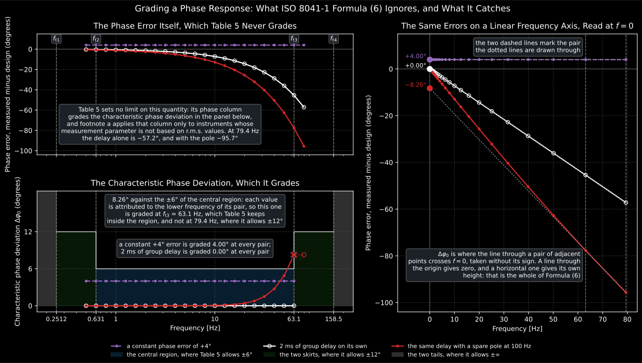
The quantity being limited is also not what it first appears. Clause 5.6.6 is explicit that the errors caused by a phase deviation depend on the rate of change of the phase error with frequency rather than on its absolute value, so the standard defines a characteristic phase deviation from the phase errors at two adjacent one-third-octave centres (Formula (6)) and puts the ±6° and ±12° limits on that instead. Annex H gives the reason: a constant group delay is a phase deviation proportional to frequency, and it affects neither the measured parameters nor , while tolerances written on the raw phase error would have to be extremely narrow to buy the same measurement accuracy.
phase_tolerance_degrees returns that band and nothing else: the limit that
applies at each frequency, with no opinion about what is being compared to it.
Computing a from a measured phase response and grading it
against the band is the next section.
8. Grading a phase response: Formula (6) and what it ignores
Section titled “8. Grading a phase response: Formula (6) and what it ignores”Formula (6) turns two adjacent phase errors into one number:
It is a slope written as an intercept. Read the two phase errors as two points
on a line against frequency; the quantity inside the bars is where that line
crosses . So a phase error that runs straight through the origin is
graded as nothing at all, and a phase error offset from the origin is graded by
the size of the offset. Formula (H.3) of the normative Annex H prints the same
quantity with the two products exchanged, which is the same number inside the
bars, and it settles where the answer belongs: N frequencies give N − 1
values, each attributed to the lower frequency of its pair. That is what
decides which Table 5 region grades a pair straddling a transition frequency.
The two invariances are worth seeing rather than reading about, because they are the whole justification for a criterion that looks so indirect:
import numpy as npfrom phonometry import vibration
bands = np.arange(-10, 27)frequencies = 10.0 ** (bands / 10.0)
# A constant phase error is graded at face value.constant = vibration.characteristic_phase_deviation(    frequencies, np.full(frequencies.shape, 4.0))print(round(float(constant.min()), 6), round(float(constant.max()), 6))# 4.0 4.0
# A phase error proportional to frequency is a constant group delay, and it# is graded as zero however large it gets. This one is 2 ms.delay_deg = -360.0 * frequencies * 2e-3print(round(float(delay_deg.min()), 1), round(float(delay_deg.max()), 1))# -286.6 -0.1ramp = vibration.characteristic_phase_deviation(frequencies, delay_deg)print(float(np.max(ramp)) < 1e-10)   # True
A phase error of up to 287 degrees, graded as zero. NOTE 1 of H.2.1 says exactly that about a constant group delay: it “would probably far exceed the tolerances on phase deviation, but would influence neither the vibration parameters to be measured nor the characteristic phase deviation values”. A meter that delays everything by the same time has changed when the waveform arrives and not what it looks like, and the peak, the MTVV and the VDV of a delayed waveform are the peak, the MTVV and the VDV. Tolerances written on the raw phase error would have to be brutally narrow to leave room for a delay every real instrument has.
The oracle. Annex B prints a phase column for the overall weighting in every one of Tables B.1 to B.9, calculated from Formula (H.1), which is the argument of the same the magnitudes come from. Those columns run down one continuous branch, from close to +180 degrees at the bottom of each table to well past −180 at the top, and the design goal is followed along that branch rather than folded into a half turn either side of zero. Five rows of Table B.8, computed rather than transcribed:
# frequencies is the one-third-octave grid of the block above.design = vibration.verify_phase_response(    "Wk", frequencies, np.zeros_like(frequencies)).design_phase_deg
for band in (-10, 0, 8, 18, 26):    index = band + 10    print(band, round(float(frequencies[index]), 4),          round(float(design[index]), 4))# -10 0.1 159.7661# 0 1.0 40.0607# 8 6.3096 -6.8409# 18 63.0957 -137.5858# 26 398.1072 -247.9414
Table B.8 prints 159.8, 40.06, −6.841, −137.6 and −247.9 in those rows. The last one is the point: −247.9 degrees is not a phase anybody’s instrument displays, it is where the branch has got to, and it is what the measurement has to arrive on too. Folding either side into destroys the delay invariance, which is the one thing the criterion exists for. H.2.3.4 g) to m) is the standard’s own recipe for rebuilding the continuous curve from wrapped phase-meter readings, and it belongs before the call rather than inside it: on a one-third-octave grid a wrap and a delay ramp are the same jump, so nothing downstream could tell them apart.
A verdict. The instrument below has two defects. One is 2 ms of group delay, which the criterion is blind to. The other is a spare pole at 100 Hz, an anti-alias filter dropped where the design goal already has its band-limiting corner, and the criterion is not blind to that at all. The grid is the nominal frequency range of a whole-body meter, on the exact centres of Formula (B.1):
bands = np.arange(-3, 20)frequencies = 10.0 ** (bands / 10.0)print(round(float(frequencies[0]), 4), round(float(frequencies[-1]), 4))# 0.5012 79.4328
design = vibration.verify_phase_response(    "Wk", frequencies, np.zeros_like(frequencies)).design_phase_degdelay = -360.0 * frequencies * 2e-3spare_pole = -np.degrees(np.arctan(frequencies / 100.0))
check = vibration.verify_phase_response(    "Wk", frequencies, design + delay + spare_pole)print(check.passes)                                                  # Falseprint(check.failing_frequencies_hz.round(2))                         # [63.1]print(round(float(check.characteristic_deviation_deg.max()), 2))     # 8.26print(round(check.peak_deviation_percent, 1))                        # 6.9
check.plot()   # the characteristic deviation inside its band (needs matplotlib)
Take the pole away and the delay alone is a phase error of up to 57 degrees that the criterion grades as zero:
delayed = vibration.verify_phase_response("Wk", frequencies, design + delay)print(round(float(delayed.deviation_deg.min()), 1), round(float(delayed.deviation_deg.max()), 1))# -57.2 -0.4print(delayed.passes) # Trueprint(float(delayed.characteristic_deviation_deg.max()) < 1e-10) # True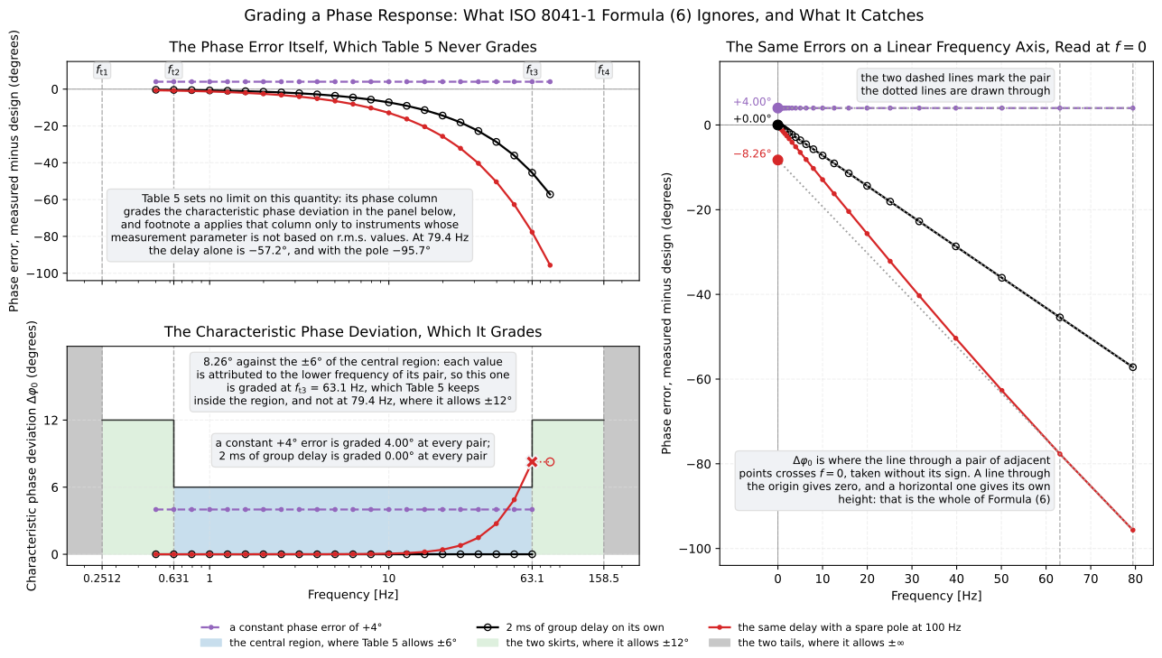
Show the code for this figure
import matplotlib.pyplot as plt
# frequencies, design, delay, spare_pole and check come from the blocks above.
# One line, for the response the section grades:check.plot()plt.show()
# The two panels that share a frequency axis, from the results' fields: the# phase error Table 5 never grades, and the characteristic deviation it does.errors = {    "a constant +4 degrees": np.full(frequencies.shape, 4.0),    "2 ms of group delay on its own": delay,    "the same delay with a spare pole at 100 Hz": delay + spare_pole,}attributed = frequencies[:-1]limit = vibration.phase_tolerance_degrees("Wk", attributed)
fig, (ax_error, ax_graded) = plt.subplots(2, 1, sharex=True, figsize=(9, 7))for label, error in errors.items():    graded = vibration.verify_phase_response("Wk", frequencies, design + error)    ax_error.semilogx(frequencies, graded.deviation_deg, marker="o", label=label)    ax_graded.semilogx(attributed, graded.characteristic_deviation_deg, marker="o")ax_graded.plot(attributed, limit, color="#1f77b4", ls="--", drawstyle="steps-post",               label="the Table 5 limit")ax_error.set_ylabel("Phase error [deg]")ax_error.legend(fontsize="small")ax_graded.set(xlabel="Frequency [Hz]", ylabel="Characteristic deviation [deg]")ax_graded.legend(fontsize="small")for ax in (ax_error, ax_graded):    ax.grid(True, which="both", alpha=0.3)plt.show()
What a phase error costs a peak reading. Annex H is normative, and Formula (H.4) is the only worked number in the whole phase argument: , followed by the sentence that for the maximum characteristic phase deviations of 12 degrees the maximum peak-value deviation is approximately 10 %. The maximum is inside the printed formula, so the answer is one number for a whole response rather than one per frequency, and it is what the worst pair costs:
print(round(vibration.peak_deviation_percent([12.0]), 2)) # 9.98print(round(vibration.peak_deviation_percent([6.0]), 2)) # 5.02That is where the ±6 degrees and ±12 degrees of Table 5 come from: a central
region held to 5 % on a peak reading and skirts held to 10 %. It is also the
6.9 % the failing meter above was charged for its 8.26 degrees, which
PhaseVerification.peak_deviation_percent computes from the worst pair.
NOTE 2 of H.2.1 fences the approximation twice, and both fences are worth
knowing. It applies to values below 30 degrees, so a larger one is passed on
with a warning; and it is a worst case that combines two components in the
most unfavourable way, so the actual peak-value deviation of a real waveform
is normally smaller.
The grid. verify_phase_response refuses a grid coarser than one third of
an octave, citing 12.11.1, which asks for a frequency-response test “in steps
of not more than one-third octave”. The reason is that the design phase is
rebuilt on the grid it is given: the branch is followed frequency to frequency,
and on a coarse grid a step of more than half a turn is indistinguishable from
the next branch. The whole design would land 360 degrees away, and Formula (6)
would turn that offset on a widely spaced pair into a handful of degrees, which
can sit comfortably inside the tolerance. The failure is silent and it can go
either way, so it is refused rather than warned about:
octaves = 2.0 ** np.arange(0.0, 7.0)try: vibration.verify_phase_response("Wk", octaves, np.zeros_like(octaves))except ValueError as error: print(error)# verify_phase_response: 'frequencies_hz' steps by a ratio of up to 2, and# ISO 8041-1:2017 12.11.1 asks for steps of not more than one third of an# octave (1.259). The design-goal phase is rebuilt on the grid it is given,# and on a coarser one it can land a whole turn away without the verdict# noticing.One last case is worth knowing about, because the verdict is right and the diagnosis is not. A measurement half a turn from the design goal at every frequency is an inverted signal, and Formula (6) grades a constant offset at face value, so it fails by 180 degrees and fails loudly. H.2.3.4 k) says the criterion “is not applicable to signal inversion” and that polarity has its own test procedure, so the verdict comes with a warning saying so: the number is real, and the fault it points at is a test this function does not perform.
9. How long the running r.m.s. takes to forget
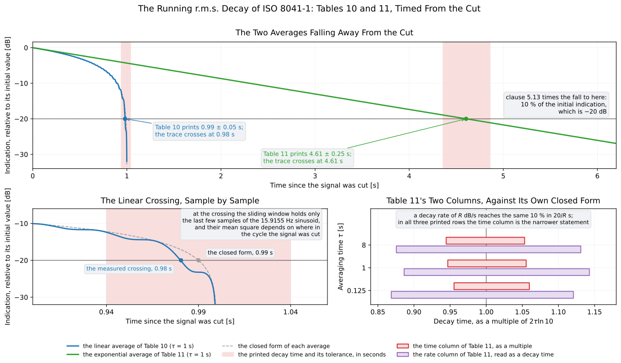
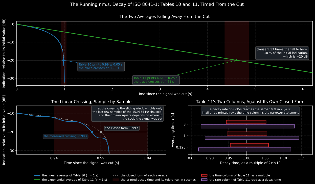
Section titled “9. How long the running r.m.s. takes to forget”Clause 5.13 is the time weighting, and its test is a stopwatch. A steady sinusoid at the reference frequency runs long enough to fill the average, at least 5 time constants for the linear one and 20 for the exponential; then it is shut off, and the time is taken from the cut to the moment the indicated value drops below 10 % of what it was. Tables 10 and 11 print that time for three time constants, with the tolerance beside it:
from phonometry import vibration
print(vibration.RUNNING_RMS_DECAY_TIME_S["linear"])# ((0.125, 0.124, 0.005), (1.0, 0.99, 0.05), (8.0, 7.92, 0.2))print(vibration.RUNNING_RMS_DECAY_TIME_S["exponential"])# ((0.125, 0.58, 0.03), (1.0, 4.61, 0.25), (8.0, 36.8, 2.0))
Both averages have a closed form, and neither is a fitted constant. The linear
average keeps the last seconds of the record, so seconds after the
cut its window still holds of the original mean square and the
indication falls as , reaching a tenth at
. The exponential average decays in power as , so
the indication falls as and reaches a tenth at
. running_rms_decay_time is those two
expressions, and they land on the printed numbers:
for method in ("linear", "exponential"): print(method, [round(vibration.running_rms_decay_time(tau, method=method), 4) for tau in (0.125, 1.0, 8.0)])# linear [0.1237, 0.99, 7.92]# exponential [0.5756, 4.6052, 36.8414]Running the test on a signal gives the same answer, which is the point of having the closed form at all. The signal below is already weighted, since the time weighting sits after the frequency weighting in the chain:
import numpy as np
fs = 2000.0cut_s = 10.0t = np.arange(int(20 * fs)) / fsa = np.sqrt(2.0) * np.sin(2 * np.pi * vibration.REFERENCE_FREQUENCY_HZ["Wk"] * t)a[t >= cut_s] = 0.0
for method in ("linear", "exponential"):    trace = vibration.running_rms(a, fs, integration_time=1.0, method=method)    initial = float(trace[int(cut_s * fs) - 1])    crossed = np.flatnonzero((t >= cut_s) & (trace < 0.1 * initial))    decay_s = float(t[crossed[0]] - cut_s)    verdict = vibration.verify_running_rms_decay(        decay_s, integration_time_s=1.0, method=method)    print(method, round(decay_s, 3), verdict.passes,          round(verdict.lower_time_s, 3), round(verdict.upper_time_s, 3))# linear 0.98 True 0.94 1.04# exponential 4.605 True 4.36 4.86
The linear reading comes out at 0.98 s rather than the 0.99 s of the closed
form, and that is the test behaving as a test rather than as arithmetic. At the
moment of the crossing the sliding window holds only the last few samples of a
sinusoid, and their mean square depends on where in the cycle the signal was
cut. The printed band is 0.99 ± 0.05 s, wide enough to absorb it, which is why
the band is what the verdict is written against and not the closed form. The
verdict keeps that row: measured_time_s, printed_time_s and tolerance_s
beside passes, the interval as lower_time_s and upper_time_s, and
.plot() draws the reading on the 10 % rule inside it.
Show the code for this figure
import matplotlib.pyplot as plt
tau = 1.0cut = int(cut_s * fs)since_cut = np.arange(t.size - cut) / fs# The 10 % of the clause, read back out of the closed form rather than typed:# the exponential average falls as exp(-t / 2 tau), so the fraction is what# that expression is worth at the time running_rms_decay_time returns.fraction = np.exp(-vibration.running_rms_decay_time(tau, method="exponential") / (2 * tau))
fig, ax = plt.subplots()for method, colour in (("linear", "#1f77b4"), ("exponential", "#2ca02c")):    trace = np.asarray(vibration.running_rms(a, fs, integration_time=tau, method=method))    relative = trace[cut:] / trace[cut - 1]    # The linear average empties one time constant after the cut, and a level    # is not defined where the mean square in the window is exactly zero.    level_db = np.full(relative.shape, np.nan)    level_db[relative > 0.0] = 20.0 * np.log10(relative[relative > 0.0])    ax.plot(since_cut, level_db, color=colour, lw=1.8, label=f"{method} average")
    # The printed band the crossing has to land in, from Table 10 or Table 11.    printed, tolerance = {        row[0]: row[1:] for row in vibration.RUNNING_RMS_DECAY_TIME_S[method]    }[tau]    ax.axvspan(printed - tolerance, printed + tolerance, color=colour, alpha=0.12)
ax.axhline(20.0 * np.log10(fraction), color="0.4", lw=1.0)ax.set(xlim=(0.0, 6.2), ylim=(-34.0, 2.0),       xlabel="Time since the signal was cut [s]",       ylabel="Indication, relative to its initial value [dB]")ax.grid(True, alpha=0.3)ax.legend()plt.show()
verify_running_rms_decay grades one printed row, and only the three time
constants the two tables print. Anything else is refused rather than judged
against a band the standard does not give:
try: vibration.verify_running_rms_decay( 2.0, integration_time_s=2.0, method="linear" )except ValueError as error: print(error)# 'integration_time_s' must be one of the time constants Tables 10 and 11# print (0.125, 1, 8 s); 2 s has no printed decay band.Why the time column and not the rate column. Table 11 prints a second way of saying the same thing, an equivalent decay rate in decibels per second, and it is deliberately not the criterion:
print(vibration.RUNNING_RMS_DECAY_RATE_DB_PER_S)# ((0.125, 31.0, 40.0), (1.0, 3.8, 4.9), (8.0, 0.48, 0.62))print(round(20 * np.log10(np.e) / 2.0, 4)) # 4.3429The closed-form rate of an exponential average is decibels per second, which for s is 4.3429 and sits in the middle of the printed 3.8 to 4.9. But that interval is 0.875 to 1.128 times the closed form, while the printed time for the same row, 4.61 ± 0.25 s, is 0.947 to 1.055 times : about half as wide, and the other two rows divide the same way. The two columns are not reciprocals of one another: the time column binds and the rate column is the looser statement of the same decay, so the verdict is written on the tighter one.
The third row of Table 2 belongs here too. It allows 2 % between the running
r.m.s. indication and the linear time-averaged r.m.s. value, both band-limited,
over any measurement time, and it is published as
RUNNING_RMS_CONSISTENCY_TOLERANCE_PERCENT. For a steady sinusoid the running
r.m.s. ripples around the time average by about 0.3 %, well inside it.
10. The saw-tooth burst, and the 228 numbers it has to reproduce
Section titled “10. The saw-tooth burst, and the 228 numbers it has to reproduce”Clause 5.9 is the one place in the whole document where ISO 8041-1 prints an oracle instead of a requirement. It defines a test signal in Table 6, and then prints in Tables 7, 8 and 9 the indications a conforming meter has to show when that signal is applied, each with the tolerance it is judged against: 228 cells in all. NOTE 1 says where they come from, and it is the sentence that makes this section possible at all: “The response to the saw-tooth signal burst is determined by digital simulation of the filter characteristics.” They are arithmetic, so a library that has the weightings and the four indication quantities can reproduce them.
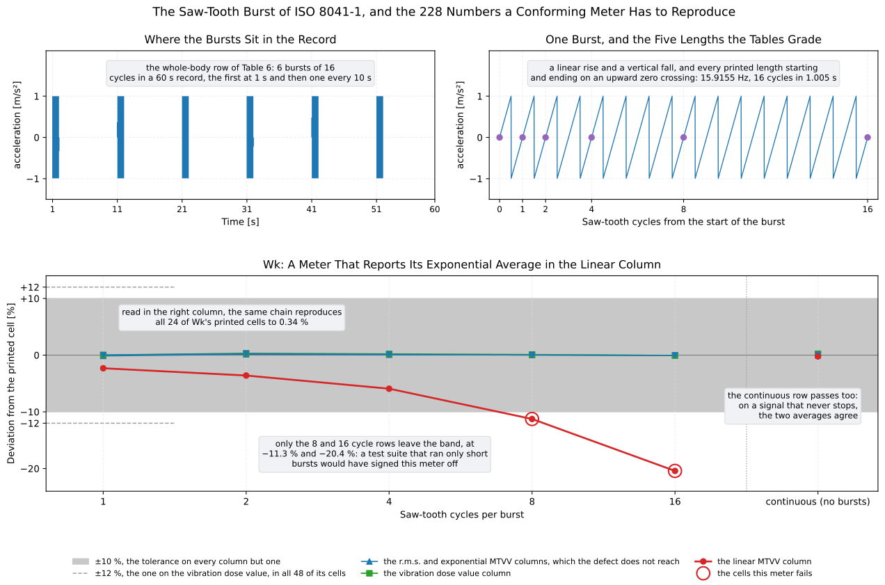
The signal. Figure 3 draws a bipolar saw-tooth of amplitude 1 m/s²: a
linear rising ramp and a vertical fall, with every burst starting at an upward
zero crossing and ending at one. That geometry carries weight rather than
decoration, because a burst started at the peak reads 28 % high on the
single-cycle row of Table 8, nearly three times its 10 % tolerance. Table 6 supplies the
rest per application, and SAWTOOTH_BURST_TESTS is that table:
import numpy as npfrom phonometry import vibration
test = vibration.SAWTOOTH_BURST_TESTS["whole-body"]print(test.weightings)# ('Wb', 'Wc', 'Wd', 'We', 'Wj', 'Wk', 'Wm')print(round(test.frequency_hz, 4), test.start_time_s, test.repeat_time_s,      test.duration_s, test.burst_count)# 15.9155 1.0 10.0 60.0 6print(test.cycle_counts, test.recommended_sampling_rate_hz)# (1, 2, 4, 8, 16) 20000.0
record = vibration.sawtooth_burst("whole-body", 2)print(record.size, np.count_nonzero(record))            # 1200000 15078print(round(float(record.max()), 4), round(float(record.min()), 4))# 0.9995 -0.9999
Six bursts of two cycles each, in a minute of otherwise silent record. The recommended sampling rate is the library’s own choice, not a normative figure: nothing in the standard prescribes one, and this is the rate at which the printed cells come back to a few tenths of a per cent.
Reproducing a row. signal_burst_indications runs the chain the standard
describes and returns the printed columns of that application’s table:
got = vibration.signal_burst_indications("whole-body", "Wk", 4)printed = vibration.SIGNAL_BURST_RESPONSE["whole-body", "Wk", 4]for column, cell in printed.items(): print(column, cell, round(got[column], 5))# rms 0.0577 0.05775# vdv 0.455 0.45597# mtvv_linear 0.182 0.18261# mtvv_exponential 0.171 0.17123Four columns because Table 8 prints four. Table 7 prints one, an r.m.s. value,
and Table 9 prints two, an r.m.s. value and a motion sickness dose value; the
column set follows the application rather than the caller. Two of Table 8’s
columns are the same MTVV computed twice, which is why mtvv grew a method:
the linear average of ISO 2631-1 Eq. (2) and the exponential average of Eq. (3)
give different answers, and the standard grades both.
verify_signal_burst_response compares a measured set of indications against
the printed cells, row by row and column by column, each against the tolerance
printed beside it:
rows = { cycles: vibration.signal_burst_indications("whole-body", "Wk", cycles) for cycles in (1, 2, 4, 8, 16, None)}check = vibration.verify_signal_burst_response("whole-body", "Wk", rows)print(check.quantities)# ('rms', 'vdv', 'mtvv_linear', 'mtvv_exponential')print(check.tolerance_percent) # [10. 12. 10. 10.]print(check.passes, round(check.worst_deviation_percent, 2)) # True 0.34None is the continuous row, which the tables print without a burst length.
The vibration dose value is the one column allowed 12 % rather than 10 %, in
all 48 of its cells.
Here is a meter that fails, and it fails in an instructive way. It computes its MTVV with an exponential average and reports it in the linear column:
swapped = {    cycles: {**row, "mtvv_linear": row["mtvv_exponential"]}    for cycles, row in rows.items()}verdict = vibration.verify_signal_burst_response("whole-body", "Wk", swapped)print(verdict.passes, round(verdict.worst_deviation_percent, 1))   # False -20.4print(verdict.deviation_percent[:, 2].round(1))# [ -2.3  -3.6  -5.9 -11.3 -20.4  -0.2]print(verdict.cycle_counts)     # (1, 2, 4, 8, 16, None)
verdict.plot()   # the deviations against the printed band (needs matplotlib)
The 1, 2 and 4 cycle rows pass, the continuous row passes because the two averages agree on a signal that never stops, and the 8 and 16 cycle rows are where the confusion shows. A test suite that ran only short bursts would have signed the instrument off.
Show the code for this figure
import matplotlib.pyplot as pltimport numpy as np
# One line, from the verdict above:verdict.plot()plt.show()
# By hand, from the result's fields: one series per printed column of Table 8,# inside the band the same table allows, with the wider allowance of the# vibration dose value drawn as a pair of edges rather than as a second band# under every column. The continuous row sits past a dotted rule with no line# drawn into it, as it does in the figure: Table 6 gives it no burst length,# so joining it to the 16 cycle point would draw a trend across a gap that# does not exist.positions = np.arange(len(verdict.cycle_counts))inner = float(np.min(verdict.tolerance_percent))outer = float(np.max(verdict.tolerance_percent))
fig, ax = plt.subplots(figsize=(9.0, 4.5))ax.axhspan(-inner, inner, color="#9e9e9e", alpha=0.25,           label=f"±{inner:.0f} % on every column but one")# The wider pair belongs to the vibration dose value alone, so it is drawn as# a stub at the edge rather than across the panel, where a rule at -12 % would# pass through the ringed 8 cycle cell of a column it does not apply to.for edge in (-outer, outer):    ax.plot([positions[0] - 0.4, positions[0] + 0.4], [edge, edge],            color="#9e9e9e", ls="--", lw=1.0)ax.axhline(0.0, color="black", lw=0.8, alpha=0.4)ax.axvline(positions[-1] - 0.5, color="#9e9e9e", ls=":", lw=1.0)for index, quantity in enumerate(verdict.quantities):    deviations = verdict.deviation_percent[:, index]    burst_rows, = ax.plot(positions[:-1], deviations[:-1], marker="o",                          label=quantity)    ax.plot(positions[-1:], deviations[-1:], marker="o", ls="none",            color=burst_rows.get_color())outside = ~verdict.within_toleranceax.plot(positions[np.nonzero(outside)[0]], verdict.deviation_percent[outside],        "o", markersize=14, markerfacecolor="none", markeredgecolor="#d62728",        ls="none", label="the cells this meter fails")ax.set_xticks(positions)ax.set_xticklabels(["1", "2", "4", "8", "16", "continuous"])ax.set(xlabel="Saw-tooth cycles per burst",       ylabel="Deviation from the printed cell [%]")ax.grid(True, axis="x", alpha=0.3)ax.legend(fontsize="small")plt.show()
Two conventions the tables do not print. The printed cells are the output of a simulation nobody published, so two readings of the same clause give two different sets of numbers, and this branch chose by measuring which reading reproduces the page. Both are decisions rather than deductions, and both are worth stating plainly.
The continuous row starts at t = 0 and fills the printed duration. It does not start at the Table 6 start time, which applies to the bursts. Read from zero, the band-limiting continuous cell of Table 7 comes out at 0.5649 against the 0.565 printed; read from the start time it comes out at 0.5602:
test = vibration.SAWTOOTH_BURST_TESTS["hand-arm"]fs = test.recommended_sampling_rate_hzprinted = vibration.SIGNAL_BURST_RESPONSE[    "hand-arm", vibration.BAND_LIMITING, None]["rms"]from_zero = vibration.signal_burst_indications(    "hand-arm", vibration.BAND_LIMITING, None)["rms"]print(printed, round(from_zero, 4), round((from_zero / printed - 1) * 100, 2))# 0.565 0.5649 -0.02
# The reading the branch rejected: the same saw-tooth started late.samples = round(test.duration_s * fs)t = np.arange(samples) / fselapsed = test.frequency_hz * (t - test.start_time_s)saw = 2.0 * np.mod(elapsed + 0.5, 1.0) - 1.0late = np.where(t >= test.start_time_s, saw, 0.0)padded = np.concatenate([late, np.zeros(samples)])weighted = vibration.apply_band_limiting(    padded, fs, name=test.band_limiting_weighting)from_start = float(np.sqrt(np.mean(weighted[:samples] ** 2)))print(round(from_start, 4), round((from_start / printed - 1) * 100, 2))# 0.5602 -0.86
Notice that both readings pass, since the tolerance is 10 % and the worse of the two misses by 0.86 %. That is exactly why the question had to be settled by which one reproduces the printed digits: the tolerance is far too wide to decide it.
The filtering is zero state. apply_weighting multiplies in the frequency
domain without padding, which is a circular convolution, and its own
documentation says so. On a burst record that hardly matters. On the continuous
row it wraps the tail of the record onto its front and erases the switch-on
transient, which is precisely what the linear MTVV of that row is built to
catch. The burst verification pads the record with zeros first and keeps the
front, which is a filter switched on at t = 0 with nothing stored in it:
fs = vibration.SAWTOOTH_BURST_TESTS["whole-body"].recommended_sampling_rate_hzrecord = vibration.sawtooth_burst("whole-body", None)
for name in ("Wc", "Wm", "Wd", "We"):    cell = vibration.SIGNAL_BURST_RESPONSE["whole-body", name, None]    printed = cell["mtvv_linear"]    wrapped = vibration.apply_weighting(record, fs, name=name)    circular = vibration.mtvv(wrapped, fs)    from_rest = vibration.signal_burst_indications(        "whole-body", name, None    )["mtvv_linear"]    print(name,          round((circular / printed - 1) * 100, 2),          round((from_rest / printed - 1) * 100, 2))# Wc -0.81 -0.17# Wm -1.1 -0.31# Wd -3.24 -0.36# We -5.19 -0.52
Up to 5.2 % on four cells, from a choice about what the filter had in it before
the record began. The default of apply_weighting is deliberately left alone:
the padding belongs to this test, not to every weighted signal, and a reader
who needs it elsewhere pads the record with zeros first and drops the padding
after, which is what the previous snippet does.
What the reproduction is worth, across all three applications and all 228 printed cells, is 2.3 % at worst against printed tolerances of 10 % and 12 %. And what a pass means is still narrow: the time response of one weighting chain matches the printed table on the day it was measured.
11. The personal meter of ISO 8041-2
Section titled “11. The personal meter of ISO 8041-2”Everything above is ISO 8041-1, the general-purpose meter an engineer carries to a machine or a seat. ISO 8041-2:2021 specifies the other instrument a human-vibration survey uses, the personal vibration exposure meter (PVEM): the one left unattended to log a worker’s exposure through a full working day, at least 12 h without anyone touching it (5.1 and 5.12), with its transducer fitted to the worker, to the seat, or to the machine or power tool (5.1.2 and 5.1.3). It measures the same quantities through the same weightings, and Part 2 does not write a second set of tables for it. It prints the Part 1 tables again wherever it can, so the question for this section is which of the numbers above a PVEM is held to, and which are its own.
The same burst, to the digit. Part 2 5.9 repeats the saw-tooth signal
burst of section 10. Its Table 6 defines the same test signal, and its
Tables 7, 8 and 9 print 228 indications with a tolerance beside each. Read off
the Part 2 pages and set beside SIGNAL_BURST_RESPONSE, every one of the 228
indications and every one of the 228 tolerances is the Part 1 number, and
12.13 of Part 2 grades them with the same sentence and the same 3 % maximum
uncertainty. So one implementation serves both parts: the snippets of
section 10 are the Part 2 test as they are written, and the conformance report
grades the library against the Part 2 page in a section of its own, which also
holds every Part 2 cell against its Part 1 twin.
from phonometry import vibration
# The table section 10 reproduces is the Part 2 table too: 72 printed lines# and 228 cells, the Wk row of Table 8 among them.cells = vibration.SIGNAL_BURST_RESPONSEprint(len(cells), sum(len(row) for row in cells.values()))   # 72 228print(dict(cells["whole-body", "Wk", 4]))# {'rms': 0.0577, 'vdv': 0.455, 'mtvv_linear': 0.182, 'mtvv_exponential': 0.171}
Table 2 loses a row. The tolerances of indication of Part 2 are the first
two rows of the Part 1 table, number for number: 4 % on the indication at the
reference frequency, 5 % for low-frequency whole-body vibration, and 3 %
between a frequency-weighted indication and the band-limited one times the
weighting factor. The third row, the 2 % between the running r.m.s. and the
linear average, is gone, because Part 2 5.13 reads in full “Not applicable for
PVEM”. Nor does Part 2 print a decay-time table, so section 9 has no
counterpart in it. The running r.m.s. does not leave the instrument
altogether, though: 5.1.2 still lets a whole-body PVEM report the MTVV, the
largest value its running r.m.s. reaches, and Table 8 grades that MTVV in
the burst exactly as section 10 does.
PVEM_INDICATION_TOLERANCES_PERCENT is that table, so a check that walks it
grades a PVEM on what Part 2 prints and on nothing else:
from phonometry import vibration
print(dict(vibration.PVEM_INDICATION_TOLERANCES_PERCENT))# {'indication': 4.0, 'low-frequency indication': 5.0, 'weighting consistency': 3.0}
# The row Part 2 does not print stays where Part 1 put it.print(vibration.RUNNING_RMS_CONSISTENCY_TOLERANCE_PERCENT)   # 2.0
Two paragraphs of Part 2 12.7 came over from Part 1 unchanged, and neither
fits the meter it now describes. The weighting-consistency test still points
at “the appropriate weighting factor (see Table 1)”, and the Part 2 Table 1
still prints 0,388 8 for Wf, so the caveat of section 6 applies to a PVEM
word for word: band_limited_weighting_factor is the factor that makes the row
satisfiable. And the paragraph after it still grades “each time weighting”
against “the tolerance limits of Table 2”, whose time-weighting row Part 2 no
longer prints. Both are in the errata registry.
Its own uncertainties. Part 2 prints the maximum expanded uncertainty each of its test clauses allows a laboratory, and in clause 12, pattern evaluation, every figure is the one Part 1 prints under the same number: 4,5 % for the mechanical frequency response of 12.11.2, 3 % for the electrical one of 12.11.3, 5 % for the overall response of 12.11.4, 3 % for the signal burst of 12.13. Clause 13 is where the two documents part. Part 2 has no validation of a one-off instrument, which is clause 13 of Part 1, and its periodic verification is clause 13 rather than 14: the 13.9 of Part 2 is the 5 % of a periodic verification, the counterpart of the Part 1 14.9, while the 13.9 of Part 1 is the 2 % of a different test. A clause number names a different test in each document, which is why the two tables are kept apart:
from phonometry import vibration
pvem = vibration.PVEM_MAX_EXPANDED_UNCERTAINTY_PERCENTgeneral = vibration.MAX_EXPANDED_UNCERTAINTY_PERCENTfor clause in ("12.11.2", "12.11.3", "12.11.4", "12.13"):    print(clause, pvem[clause], general[clause])# 12.11.2 4.5 4.5# 12.11.3 3.0 3.0# 12.11.4 5.0 5.0# 12.13 3.0 3.0print(pvem["13.9"], general["13.9"], general["14.9"])   # 5.0 2.0 5.0print(sorted(set(general) - set(pvem)))# ['13.11', '13.14', '13.15', '14.9']print(vibration.ISO8041_COVERAGE_FACTOR)                # 2.0
The decision rule of section 4 does not change: Part 2 12.1 and 13.1 print the
sentence and the coverage factor Part 1 prints, so verify_weighting with the
laboratory’s own expanded_uncertainty_percent is the PVEM verdict too, with
the Part 2 figure as the ceiling on what the laboratory may declare.
What Part 2 adds beyond these tables is not here. The arithmetic of its 12.11, Formulae (9) to (13), splits a frequency-response error between the transducer and the electrical part of the instrument and combines the apparent error with the laboratory’s uncertainty; the logging test of 12.22 runs the meter for 12 h, with a shaker run at each end, and reads its log file sample by sample; and logging, operator detection, the detection of transient artefacts (Annex A) and contact force (Annex B) are properties of the hardware.
12. The same check on the other side of the fence
Section titled “12. The same check on the other side of the fence”A sound level meter gets exactly this treatment, from a different committee
and in a different unit. IEC 61672-1 prints design goals for the A, C and Z
weightings and acceptance limits around them, and
verify_weighting_class turns a response
into a verdict against them. The two verifiers are the same idea applied on
either side of the acoustics-vibration fence:
import numpy as npfrom phonometry import filters, vibration
# Sound: a weighting filter this library designed, against IEC 61672-1 Table 3.wf = filters.WeightingFilter(48000, "A")print(filters.verify_weighting_class(wf).overall_class)   # 1
# Vibration: the bench sweep of section 2, against ISO 8041-1 Tables 4 and 5.sweep = 10.0 ** (np.array([-3, 0, 3, 6, 9, 12, 15, 18, 19]) / 10.0)read = np.array([0.4314, 0.4969, 0.5466, 0.9937, 1.068,                 0.7897, 0.3427, 0.1894, 0.1366])print(vibration.verify_weighting("Wk", sweep, read).passes)   # False
Three differences are worth naming, because they are the ones that trip a reader moving between the two pages.
There are no classes. IEC 61672-1 specifies two performance categories, and the verdict is which of them a response meets. ISO 8041-1 has none: it prints one set of tolerances, and the verdict is pass or fail against it.
The limits are percentages, not decibels. ISO 8041-1 writes its magnitude tolerances as percentages of the weighting factor, and the library keeps them that way. The informative Annex B prints the decibel equivalents beside them, +1 dB / −1 dB in the central region and +2 dB / −2 dB in the skirts, but the percentage is what the requirement is written in.
They are graded against different things. verify_weighting_class reads a
digital filter this library built and reports whether that design fits the
mask, so any measurement made in software inherits the verdict.
verify_weighting is handed numbers from a bench, and its verdict belongs to
that measurement of that instrument, on the day it was made. Neither is a
pattern evaluation, a periodic verification or an in situ check, and neither
has a microphone, a transducer or a serial number.
Compliance and verification
is the map of every verifier in the library and of where each one’s claim
ends.
What this guide covers
Section titled “What this guide covers”Covered
The tolerance band on a frequency weighting: the four transition frequencies of Table 4 built from their printed exponents, the three distinct pairs of limits Table 5 carries across them, and the verdict of
verify_weightingon a measured response, with the testing laboratory’s expanded uncertainty extending the deviation as 13.1 and 14.1 require.The characteristic phase deviation of Formula (6), computed on the grid 12.11.1 asks for and graded against the phase column of Table 5, with the peak cost of Formula (H.4) beside it.
The band-limiting stage on its own, the running r.m.s. decay times of Tables 10 and 11 in closed form, and the 228 saw-tooth burst indications of Tables 7 to 9 reproduced from the signal Table 6 defines.
The reference conditions of Table 1 and the tolerance of indication of Table 2, published as the window an indication has to land in. They are published, not checked: reading a display is a bench measurement.
The personal vibration exposure meter of ISO 8041-2:2021: its 228 burst cells of Tables 7 to 9, the Part 1 cells to the digit, graded in the conformance report against the Part 2 page; its two-row Table 2; and the maximum expanded uncertainties its clauses 12 and 13 print.
Not covered
No bench, anywhere. Every criterion here is one side of a comparison whose other side somebody has to measure on hardware. Accuracy of indication, linearity, instrument noise, overload, cross-talk, transducer characteristics, mounting and the whole environmental and electromagnetic clause are not implemented and are not implementable here.
No conformity verdict for an instrument. A pass on any clause of this page is a statement about that clause. Pattern evaluation, periodic verification and the in situ check are procedures on a physical meter, and nothing here carries a serial number.
The rest of ISO 8041-2. The frequency-response arithmetic of its 12.11 (Formulae (9) to (13)), the 12 h logging test of 12.22, and the logging, operator detection, artefact detection (Annex A) and contact force (Annex B) clauses are not implemented.
References
Section titled “References”- Griffin, M. J. (1996). Handbook of human vibration. Academic Press. ISBN 978-0-12-303041-2. The measurement chain behind the specification: transducers, mounting, frequency weighting and the instrumentation practice the standard writes requirements for.
- International Organization for Standardization. (2017). Human response to vibration — Measuring instrumentation — Part 1: General purpose vibration meters (ISO 8041-1:2017). The three levels of performance testing (clause 1), the reference environmental conditions (clause 4), the reference vibration values and frequencies of Table 1, the three rows of Table 2, the weighting parameters of Table 3 and the transfer functions of 5.6, the transition frequencies of Table 4 and the tolerances of Table 5 with their footnote a, the characteristic phase deviation of Formula (6), the saw-tooth signal burst of 5.9 with its Table 6 and the printed responses of Tables 7 to 9, the running r.m.s. time averaging of 5.13 with Tables 10 and 11, the maximum expanded uncertainties of 12.1 and the test grid of 12.11.1, the demonstration of compliance of 13.1 and 14.1, the tabulated design-goal weightings and phases of Annex B, and the phase argument of Annex H with its Formulae (H.1), (H.3) and (H.4). The design and type-test clauses that need a bench are not implemented: a pass on any clause here is a statement about that clause and never a conformity certificate for an instrument.
- International Organization for Standardization. (2021). Human response to vibration — Measuring instrumentation — Part 2: Personal vibration exposure meters (ISO 8041-2:2021). The personal vibration exposure meter: the 12 h of 5.1 and 5.12, Table 2 with its two rows and the "Not applicable for PVEM" of 5.13, the saw-tooth signal burst of 5.9 with its Table 6 and the printed responses of Tables 7 to 9, the maximum expanded uncertainties of clauses 12 and 13, and the decision rule of 12.1 and 13.1. The frequency-response arithmetic of 12.11 and the 12 h logging test of 12.22 are not implemented.