Predicting railway vibration (E DIN 45672-3)
Standards: E DIN 45672E DIN 4150
DIN 45672-1 measures next to a line and Part 2 reduces what was measured. Part 3, which has only ever existed as the draft of February 2023, answers the question that comes before both: a line is planned, or a building next to one, and someone has to say how much the floors will move before there is anything to measure. The answer is a third-octave velocity spectrum on a floor, built by adding what is known about the source, the ground and the building, and from it the two numbers DIN 4150-2 judges.
1. A spectrum is a sum of what is known
Section titled “1. A spectrum is a sum of what is known”Formula (1) is the whole method in one line. The level in each band on the floor is the emission of the line at some known point, plus what the ground does between that point and the building, plus what the foundation does on the way in, plus what the floor does on top, plus whatever mitigation takes away:
L_v(f) = L_v,E(f) + ΔL_v,BB(f) + ΔL_v,FB(f) + ΔL_v,DF(f) + D_e(f)Every term is added as printed, so a mitigation goes in with a minus sign. The example of Annex C predicts a tram at 50 km/h for a building 7 m from the track, on a concrete floor with a natural frequency of 20 Hz; its emission spectrum was already taken at a foundation, so the foundation term is zero.
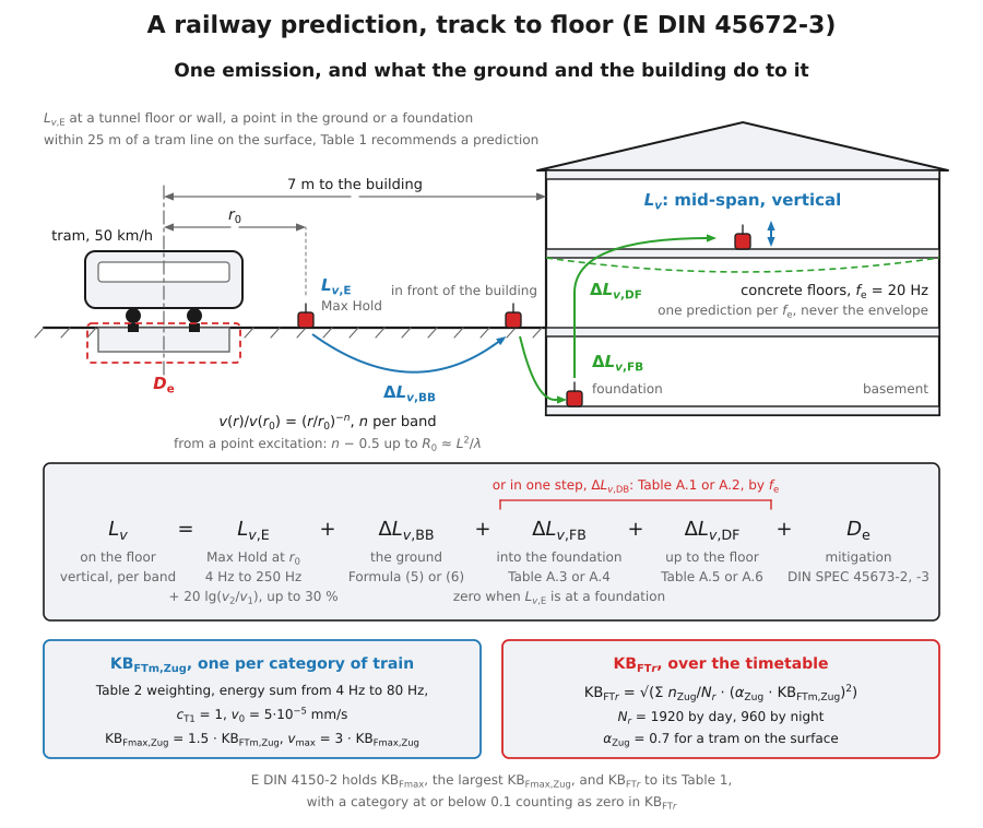
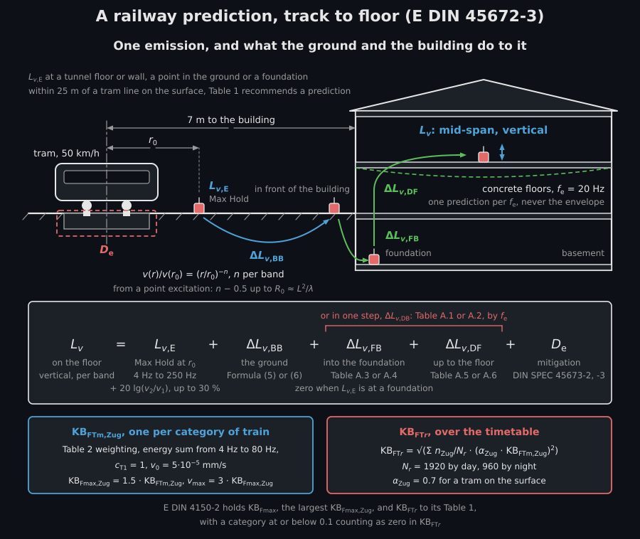
Where each term of Formula (1) belongs, from the track to the middle of a floor, and the two quantities Clause 7 turns the spectrum into for DIN 4150-2.
import numpy as np
from phonometry import vibration
# Annex C, Table C.1: the emission at the foundation, the ground for the# difference in distance, and the floor at 20 Hz, 4 Hz to 250 Hz.emission = np.array([26.0, 27.0, 37.0, 54.0, 56.0, 57.0, 56.0, 57.0, 58.0, 58.0,                     52.0, 52.0, 60.0, 58.0, 49.0, 45.0, 45.0, 33.0, 28.0])ground = np.array([0.9, 0.9, 0.9, 1.1, 1.1, 1.2, 1.3, 1.3, 1.4, 1.6,                   1.7, 2.0, 2.2, 2.6, 3.0, 3.5, 3.1, 2.8, 2.4])floor = np.array([1.9, 2.3, 3.1, 3.5, 5.0, 6.9, 11.5, 17.3, 10.0, 5.4,                  1.9, 1.5, -0.8, -2.3, -3.8, -5.4, -6.5, -8.1, -9.6])
on_floor = vibration.predict_floor_spectrum(emission, ground_db=ground, floor_db=floor)print(np.round(on_floor[:4], 1))  # [28.8 30.2 41.  58.6]print(f"{vibration.band_sum_level(on_floor):.1f} dB")  # 78.1 dB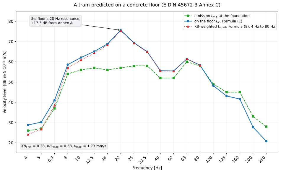
Figure code
import numpy as np
from phonometry import vibration
emission = np.array([26.0, 27.0, 37.0, 54.0, 56.0, 57.0, 56.0, 57.0, 58.0, 58.0,                     52.0, 52.0, 60.0, 58.0, 49.0, 45.0, 45.0, 33.0, 28.0])ground = np.array([0.9, 0.9, 0.9, 1.1, 1.1, 1.2, 1.3, 1.3, 1.4, 1.6,                   1.7, 2.0, 2.2, 2.6, 3.0, 3.5, 3.1, 2.8, 2.4])floor = np.array([1.9, 2.3, 3.1, 3.5, 5.0, 6.9, 11.5, 17.3, 10.0, 5.4,                  1.9, 1.5, -0.8, -2.3, -3.8, -5.4, -6.5, -8.1, -9.6])prediction = vibration.predict_train_category(emission, ground_db=ground, floor_db=floor)ax = prediction.plot()
2. Where each term comes from
Section titled “2. Where each term comes from”The emission (Clause 5.2) is a Max Hold spectrum of the kind of train, measured under traffic at a known distance, from 4 Hz to 250 Hz. A spectrum taken at one speed is carried to another of the same kind of train by 20 lg of the ratio (Formula (3)), for a change of up to 30 %; beyond that the frequencies bound to a length, the sleeper passing first, move with the speed while the resonances do not, and the shift is refused.
from phonometry import vibration
shifted = vibration.rescale_emission_for_speed([50.0], speed_from_km_h=50.0, speed_to_km_h=60.0)print(f"{shifted[0]:.2f} dB")  # 51.58 dB
The ground (Clause 5.3) is geometric spreading times material damping.
The ratio of the velocity at the building to that at the reference distance
is (r / r₀)^-n · exp(-α_R (r - r₀)) (Formula (5)) with α_R = 2π f D / c_s,
the damping ratio of the ground over the wavelength, or a power law alone
with an exponent measured per band (Formula (6)); the level difference is
20 lg of it (Formula (4)). On the surface the exponent is usually 0,2 to 0,4.
from phonometry import vibration
delta = vibration.ground_transmission_db(    [8.0, 31.5, 125.0],    distance_m=25.0,    reference_distance_m=8.0,    exponent=0.3,    damping_ratio=0.03,    shear_wave_speed_m_s=200.0,)print(delta.round(1))  # [ -4.1  -7.4 -20.4]
The building (Clause 5.4, Annex A) is six tables from extensive building measurements, which are the standard’s real content. Ground to foundation for a basement or a ground floor (Tables A.3 and A.4), as a mean with the deviation either way; foundation to floor for concrete or timber floors against the ratio of the band to the natural frequency of the floor (Tables A.5 and A.6); and, for those who would rather not split it, ground straight to the floor by that natural frequency (Tables A.1 and A.2), for every storey. The prediction is run once for each natural frequency the building may have, and never with the envelope over all of them, which the standard says overestimates considerably.
from phonometry import vibration
print(vibration.ground_to_foundation_transfer_db("basement")[:5])  # [-4.  -3.5 -3.6 -4.2 -4.2]print(vibration.foundation_to_floor_transfer_db(    [8.0, 16.0, 20.0, 40.0], floor="concrete", floor_natural_frequency_hz=20.0))  # [ 3.26  9.94 17.26  3.27]print(vibration.ground_to_floor_transfer_db("timber", floor_natural_frequency_hz=16.0)[4:8])# [ 6.03 10.07 16.    8.51]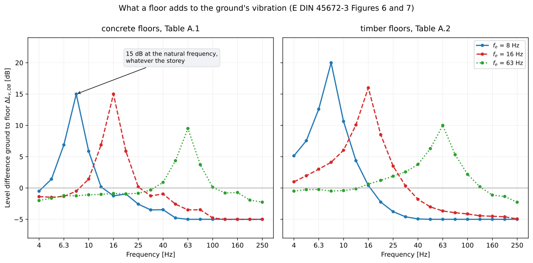
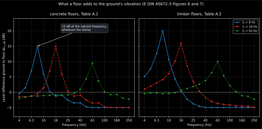
Figure code
import matplotlib.pyplot as pltimport numpy as np
from phonometry import vibration
bands = np.asarray(vibration.PREDICTION_BAND_CENTRES_HZ)positions = np.arange(bands.size)fig, axes = plt.subplots(1, 2, figsize=(11.5, 5.6), sharey=True)for ax, floor in zip(axes, ("concrete", "timber"), strict=True):    for natural in (8.0, 16.0, 63.0):        ax.plot(            positions,            vibration.ground_to_floor_transfer_db(floor, floor_natural_frequency_hz=natural),            marker="o",            label=f"$f_e$ = {natural:g} Hz",        )    ax.set_xticks(positions[::2], [f"{b:g}" for b in bands[::2]])    ax.set_title(floor)axes[1].legend()
The mitigation (Clause 5.5) is the spectral insertion loss of a track
measure from DIN SPEC 45673-2 or -3, or of any other measure determined
suitably, and it enters Formula (1) as printed, added, so as a negative
number: the argument is mitigation_db and not an insertion loss, because
an insertion loss in the sense of DIN 45672-2 Annex B is positive for a
reduction and goes in with its sign changed.
3. From the spectrum to the numbers DIN 4150-2 judges
Section titled “3. From the spectrum to the numbers DIN 4150-2 judges”Clause 7 turns the spectrum into the assessment quantities. The KB
weighting of DIN 45669-1
is printed as a table of third-octave corrections, Table 2, from 4 Hz to
80 Hz, and added to each band (Formula (8)); the weighted bands are summed;
and the sum level gives the clock maximum r.m.s. of the kind of train
(Formula (9)), KB_FTm,Zug = c_T1 · v₀ · 10^(L/20) with c_T1 = 1 for Max
Hold spectra and v₀ = 5·10⁻⁵ mm/s, the reference of the level. The value
is the KB quantity itself, because KB is the velocity in millimetres per
second. Then 1,5 times it is KB_Fmax,Zug (Formula (10)) and 3 times that
the peak velocity a DIN 4150-3
comparison wants (Formula (12)).
import numpy as np
from phonometry import vibration
emission = np.array([26.0, 27.0, 37.0, 54.0, 56.0, 57.0, 56.0, 57.0, 58.0, 58.0,                     52.0, 52.0, 60.0, 58.0, 49.0, 45.0, 45.0, 33.0, 28.0])ground = np.array([0.9, 0.9, 0.9, 1.1, 1.1, 1.2, 1.3, 1.3, 1.4, 1.6,                   1.7, 2.0, 2.2, 2.6, 3.0, 3.5, 3.1, 2.8, 2.4])floor = np.array([1.9, 2.3, 3.1, 3.5, 5.0, 6.9, 11.5, 17.3, 10.0, 5.4,                  1.9, 1.5, -0.8, -2.3, -3.8, -5.4, -6.5, -8.1, -9.6])prediction = vibration.predict_train_category(emission, ground_db=ground, floor_db=floor)print(f"{prediction.sum_level_db:.1f} dB")  # 77.7 dBprint(f"KB_FTm = {prediction.kb_ftm:.3f}")  # 0.385print(f"KB_Fmax = {prediction.kb_fmax:.3f}")  # 0.577print(f"v_max = {prediction.peak_velocity_mm_s:.2f} mm/s")  # 1.73 mm/s
The assessment vibration severity over a day’s timetable is Formula (11), the sum of Formula (6) of the draft of DIN 4150-2 with the same weighting factors, 0,7 for a tram on the surface, printed without that formula’s sentence that a category at or below 0,1 counts as zero; the library applies the sentence, since the assessment is the one the draft says it performs. With the 200 passages by day and 20 by night of the example, and the guide values of a core area, the line keeps to the requirement by day and by night:
import numpy as np
from phonometry import vibration
emission = np.array([26.0, 27.0, 37.0, 54.0, 56.0, 57.0, 56.0, 57.0, 58.0, 58.0,                     52.0, 52.0, 60.0, 58.0, 49.0, 45.0, 45.0, 33.0, 28.0])ground = np.array([0.9, 0.9, 0.9, 1.1, 1.1, 1.2, 1.3, 1.3, 1.4, 1.6,                   1.7, 2.0, 2.2, 2.6, 3.0, 3.5, 3.1, 2.8, 2.4])floor = np.array([1.9, 2.3, 3.1, 3.5, 5.0, 6.9, 11.5, 17.3, 10.0, 5.4,                  1.9, 1.5, -0.8, -2.3, -3.8, -5.4, -6.5, -8.1, -9.6])prediction = vibration.predict_train_category(emission, ground_db=ground, floor_db=floor)
alpha = vibration.train_weighting_factor("tram_metro", alignment="surface")day = vibration.train_assessment_severity([prediction.kb_ftm], [200], alpha=alpha)night = vibration.train_assessment_severity([prediction.kb_ftm], [20], alpha=alpha, time_of_day="night")print(f"KB_FTr by day {day:.3f}, by night {night:.3f}")  # 0.087, 0.039
guide = vibration.railway_guide_values("mixed", time_of_day="night")print(guide)  # GuideValues(a_u=0.1, a_o=0.6, a_r=0.07, time_of_day='night', edition='2023')verdict = vibration.assess_people_in_buildings(    prediction.kb_fmax, guide, kb_ftr=night, source="railway", edition="2023")print(verdict.complies, verdict.criterion)  # True A_r
Formula (13) goes the other way, from a level spectrum back to a velocity spectrum in micrometres per second, the form the VC curves of VDI 2038 Blatt 2 are drawn in:
from phonometry import vibration
print(vibration.velocity_spectrum_um_s([60.0, 75.6]).round(1))  # [ 50.  301.3]
4. A train is a line of points, until it is not
Section titled “4. A train is a line of points, until it is not”Annex B is for the case where the ground’s decay was measured with a point
excitation, a drop weight or a shaker, and a train is wanted. Nearer than
R₀ ≈ L² / λ (Formula (B.1)) a train of length L is a line of point sources
and its surface waves spread less than a point’s; further away it is a
point. So the exponent measured with the point is made shallower by 0,3 up
to R₀, or by 0,5 if the point fit lumped spreading and damping into one
power law, and kept as it is beyond (Formula (B.2) and Figure B.1). Within
the distances of Table 1, 25 m from a surface tram to 200 m from freight on
soft ground, the line behaviour is the rule.
from phonometry import vibration
print(vibration.point_to_line_transition_distance_m(75.0, wavelength_m=12.5))  # 450.0print(vibration.train_decay_exponent(1.0))  # 0.7print(f"{vibration.line_source_correction_db(50.0, reference_distance_m=8.0, exponent_correction=0.3):.2f} dB")  # 4.78 dBprint(vibration.RECOMMENDED_DISTANCES_M["urban"])  # {'tunnel': 20.0, 'surface': 25.0}
5. What the example gets wrong
Section titled “5. What the example gets wrong”Annex C is the only worked case, and three things in it do not follow from
the standard’s own text. Its sum level of 78,1 dB is the energy sum of all
19 bands without the weighting Clause 7.1 prescribes; the weighted sum over
4 Hz to 80 Hz is 77,7 dB, and the printed 1,81 mm/s can only be reached from
the unweighted one. Its assessment severities, 0,11 by day and 0,05 by
night, are what the printed inputs give with the factor 0,7 under the root
once instead of squared, where Formula (11) gives 0,090 and 0,040, and the
daytime verdict turns on the difference: the
example finds A_r = 0,1 exceeded, the formula finds it met. And its floor
transfer column comes from no table of Annex A, and cites Figure 3 for it
where the concrete floor is Figure 4. The conformance rows hold the chain
from the printed 78,1 dB and the formula for the printed inputs, and the
errata page has the readings, together with
a timber floor table whose lower deviation is printed above its mean, three
figure legends that name the wrong table or quantity, the sentence on a
category at or below 0,1 that Formula (11) leaves out, and an Annex A called
normative on one page and informative on its own.
The chain of Formula (1), every term added as printed; the speed rescaling of Formula (3) with its 30 % limit; the ground transmission of Formulae (4) to (6), spreading and damping with
α_R; and the mitigation as the term of Formula (1), added as printed.The six tables of Annex A read cell by cell off their pages: ground to floor for concrete and timber by natural frequency, ground to foundation for a basement and a ground floor with both deviations, foundation to floor against the ratio to the natural frequency, interpolated in decibels over the logarithm of the ratio and
nanwhere the print has none.Clause 7 entire: Table 2 as the KB weighting rounded to a tenth of a decibel, Formulae (8) to (13), and Formula (11) with the rule of the draft of DIN 4150-2 on a category at or below 0,1, which it prints without. Annex B: the transition distance, the exponent correction and the piecewise decay of Figure B.1. Table 1, the recommended distances.
Not covered
No work plan. Clause 6, the phases of a prediction from the site visit to the choice of a measure, and Annex D, its table, are procedure. The second method of Annex B, an admittance summed over the bogies of a train, is described without a formula and is not implemented.
No emission data. The standard says where an emission spectrum comes from and what it depends on; it prints one, at one foundation, and the library carries none. The spectrum is the user’s.
What this guide covers
Section titled “What this guide covers”References
Section titled “References”- Deutsches Institut für Normung. (2023). Erschütterungen im Bauwesen — Teil 2: Einwirkungen auf Menschen in Gebäuden (E DIN 4150-2:2023-08). The assessment the prediction feeds: Formula (6) and Table 2, which Part 3 takes as its Formula (11) and Table E.1.
- Deutsches Institut für Normung. (2023). Schwingungsmessung an Schienenverkehrswegen — Teil 3: Prognoseverfahren auf Basis von Terzspektren (E DIN 45672-3:2023-02). A draft: Part 3 has no published edition. Formula (1) of Clause 5.1, the speed rescaling of Formula (3), the ground transmission of Formulae (4) to (6), the six level-difference tables of Annex A, Table 2 and the chain of Clause 7 from Formula (8) to Formula (13), the recommended distances of Table 1, and Formulae (B.1) and (B.2) of Annex B. Clause 6, the phases of a prediction, and Annex D are work plans and are not implemented. Annex C is the oracle of the conformance rows.