A train passing a house puts vibration into the ground for twenty seconds and then leaves, and the question is rarely what those twenty seconds were. It is whether the vibration at the building is more than at the track wall, whether the mat under the ballast changed anything, or whether the freight trains of the night are worse than the passenger trains of the day. Every one of those compares two numbers, and two numbers can only be compared if they were formed the same way.
That is what DIN 45672 is for. Part 1 says how to measure next to a railway: where the transducers go, which directions, which trains, what the report has to contain. Part 2 says how to reduce the record once it exists, and it is the part this page implements, with the meter of DIN 45669-1 in its 4 Hz to 315 Hz railway working range. Neither part says what the result may be: the assessment is DIN 4150-2 for people and DIN 4150-3 for buildings.
1. Three stretches of one record
Section titled “1. Three stretches of one record”The first thing Part 2 does is cut the record into three stretches, and every quantity after that carries the index of the one it was read over (Clause 5).
T₁, about four seconds with the largest vibration in its middle. It is where the characteristic values of the passage are read. A short or fast train often needs less, and thenT₁may be as long asT₂and no longer.T₂, the passage itself: the time a train takes to cross an imaginary measuring section. Experience, the standard says, puts its start where the amplitude reaches about a quarter of the most frequent maxima of the passage and its end where it falls back to the same value. That is a judgement about the record, so the library asks for it rather than guessing it.T₃, the whole event, quiet approach and departure included. It is the one the energy of the passage is formed over.
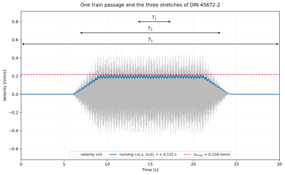
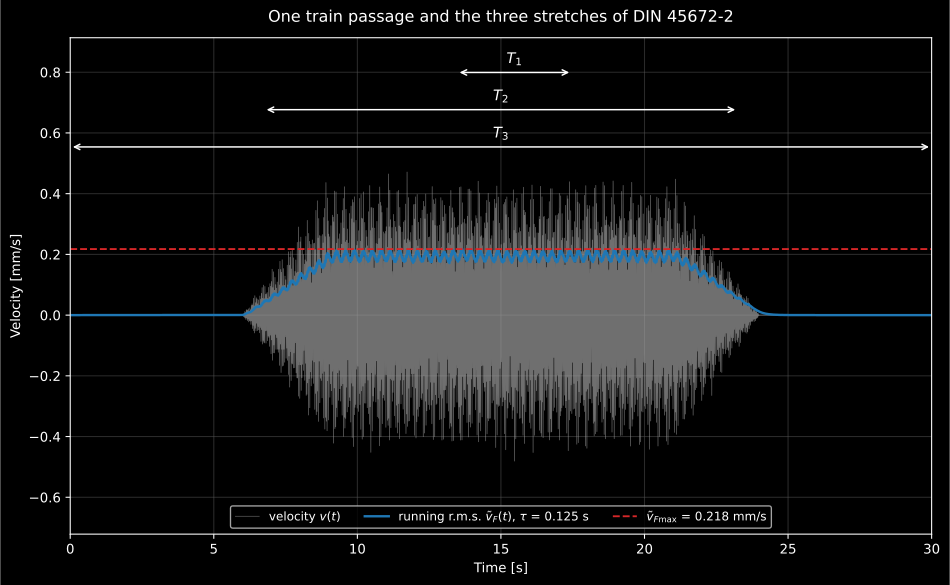
Figure code
import numpy as np
from phonometry import vibration
fs_hz = 2048t = np.arange(30 * fs_hz) / fs_hzrng = np.random.default_rng(7)envelope = np.clip((t - 6) / 3, 0, 1) * np.clip((24 - t) / 3, 0, 1)bogies = 1 + 0.5 * np.sin(2 * np.pi * 1.6 * t) ** 2record = envelope * bogies * (    0.20 * np.sin(2 * np.pi * 40 * t)    + 0.08 * np.sin(2 * np.pi * 63 * t + 1.0)    + 0.03 * rng.standard_normal(t.size))
passage = vibration.evaluate_train_passage(record, fs_hz, t2_s=(6.75, 23.25))passage.plot()
The record above is synthetic and shaped like a real one: the envelope of a
train arriving and leaving, a pulse per bogie, a sleeper-passing tone at 40 Hz,
a floor resonance at 63 Hz and some broadband noise. Its T₂ starts where the
envelope reaches a quarter, 6,75 s, and ends where it falls back, 23,25 s:
import numpy as np
from phonometry import vibration
fs_hz = 2048t = np.arange(30 * fs_hz) / fs_hzrng = np.random.default_rng(7)envelope = np.clip((t - 6) / 3, 0, 1) * np.clip((24 - t) / 3, 0, 1)bogies = 1 + 0.5 * np.sin(2 * np.pi * 1.6 * t) ** 2record = envelope * bogies * (    0.20 * np.sin(2 * np.pi * 40 * t)    + 0.08 * np.sin(2 * np.pi * 63 * t + 1.0)    + 0.03 * rng.standard_normal(t.size))
passage = vibration.evaluate_train_passage(record, fs_hz, t2_s=(6.75, 23.25))for name, (start, end), rms in zip(    ("T1", "T2", "T3"), passage.intervals_s, passage.interval_rms_mm_s):    print(f"{name}: {start:5.2f} s to {end:5.2f} s, r.m.s. {rms:.4f} mm/s")# T1: 13.47 s to 17.47 s, r.m.s. 0.1945 mm/s# T2:  6.75 s to 23.25 s, r.m.s. 0.1783 mm/s# T3:  0.00 s to 30.00 s, r.m.s. 0.1324 mm/sprint(f"v_max {passage.peak_velocity_mm_s:.3f} mm/s")        # 0.481 mm/sprint(f"v_Fmax {passage.running_rms_max_mm_s:.3f} mm/s")     # 0.218 mm/sprint(f"KB_Fmax {passage.kbf_max:.3f}")                      # 0.216
Before anything is read, the record goes through the band limitation of the
DIN 45669-1 railway range, as it does inside the meter. That is why a record
has to be the velocity the transducer gives, and why KB_Fmax, the number
DIN 4150-2 judges people by, comes out of the same call as the rest.
2. The running r.m.s., and the fourteen per cent that is seven
Section titled “2. The running r.m.s., and the fourteen per cent that is seven”The running r.m.s. of Formula (1) is the exponential average a sound level
meter calls Fast, τ = 125 ms, and its level against v₀ = 5·10⁻⁸ m/s is the
velocity level of Formula (2). Beware the reference: DIN 45672-2 defines this
5·10⁻⁸ m/s itself, without naming a source. It is the 50 nm/s that note b of
ISO 1683:2015 Table 3 says is also used for structure-borne sound, not the
1 nm/s of the main row of that table, so the same vibration is 34 dB apart
under the two.
import numpy as np
from phonometry import vibration
fs_hz = 2048t = np.arange(3 * fs_hz) / fs_hzone_mm_s_rms = np.sqrt(2) * np.sin(2 * np.pi * 40 * t)level = vibration.running_velocity_level(one_mm_s_rms, fs_hz)print(f"{level[-fs_hz:].mean():.2f} dB")  # 86.02 dB
The average starts from rest, so the first stretch of any record reads low,
and Clause 4 says why that matters: the averaging has to be running before the
train arrives. It quotes the cost as 14 % after 2τ and 2 % after 4τ, and
those are the shortfalls of the mean square, e⁻² and e⁻⁴. The running
r.m.s. the sentence is about, and the one its own Figure 3 draws, is short by
7 % and 0,9 %. The advice stands; the size of the error is overstated by a
factor of two, and the errata page has the
detail.
3. The event value, and an hour of trains
Section titled “3. The event value, and an hour of trains”The quantity a passage is summarised by is its event value (Formula (8)): the interval r.m.s. of the whole event referred to one hour,
v_E = ṽ₃ · √(T₃ / 3600 s)which is the constant velocity that, held for an hour, carries the energy the passage carried. Its level (Formula (9)) is the same thing in decibels, and because each event value is already the energy of a passage spread over the same hour, the passages of an hour add in square (Formula (10)):
from phonometry import vibration
one = vibration.event_velocity(0.1324, 30.0)print(f"one passage: v_E = {one:.5f} mm/s")  # 0.01209 mm/sprint(f"L_vE = {vibration.event_velocity_level(0.1324, 30.0):.2f} dB")  # 47.67 dB
six = vibration.combined_event_velocity([one] * 6)print(f"six in an hour: {six:.5f} mm/s")  # 0.02961 mm/s, sqrt(6) times one
That is the number to compare between two hours of traffic, and it is why
T₃ includes the quiet ends: they carry no energy, and the hour does not care
how long the record ran.
4. Third octaves: the spectra of Figure 6
Section titled “4. Third octaves: the spectra of Figure 6”Clause 7.2 analyses the passage in third octaves from 4 Hz to at least 315 Hz,
and prints two spectra as the result: the interval level over T₂
(Formula (6)), the running r.m.s. of each band averaged over the passage, and
the maximum level over T₃ (Formula (7)), the largest value the running
r.m.s. of each band reaches. The gap between them is the crest of the band:
wide where the vibration comes in bursts, narrow where it is steady.
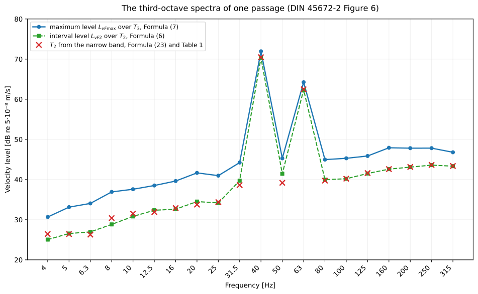
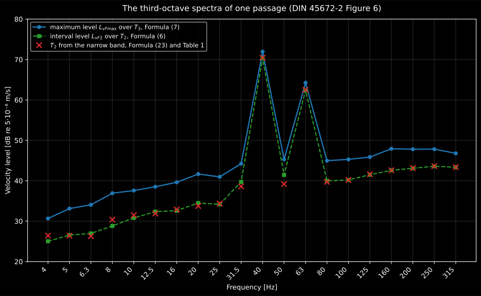
Figure code
import numpy as np
from phonometry import vibration
fs_hz = 2048t = np.arange(30 * fs_hz) / fs_hzrng = np.random.default_rng(7)envelope = np.clip((t - 6) / 3, 0, 1) * np.clip((24 - t) / 3, 0, 1)bogies = 1 + 0.5 * np.sin(2 * np.pi * 1.6 * t) ** 2record = envelope * bogies * (    0.20 * np.sin(2 * np.pi * 40 * t)    + 0.08 * np.sin(2 * np.pi * 63 * t + 1.0)    + 0.03 * rng.standard_normal(t.size))
passage = vibration.evaluate_train_passage(record, fs_hz, t2_s=(6.75, 23.25))ax = passage.plot_spectrum()
t2 = slice(round(6.75 * fs_hz), round(23.25 * fs_hz))spectrum = vibration.narrowband_psd(passage.velocity_mm_s[t2], fs_hz)centres, rms = vibration.third_octaves_from_narrowband(    spectrum.frequencies, spectrum.psd)narrow = 20 * np.log10(rms / vibration.VELOCITY_LEVEL_REFERENCE_MM_S)positions = [list(centres).index(band) for band in passage.band_centres_hz]ax.plot(range(len(positions)), narrow[positions], "x", label="T2 from the narrow band")ax.legend()
import numpy as np
from phonometry import vibration
fs_hz = 2048t = np.arange(30 * fs_hz) / fs_hzrng = np.random.default_rng(7)envelope = np.clip((t - 6) / 3, 0, 1) * np.clip((24 - t) / 3, 0, 1)bogies = 1 + 0.5 * np.sin(2 * np.pi * 1.6 * t) ** 2record = envelope * bogies * ( 0.20 * np.sin(2 * np.pi * 40 * t) + 0.08 * np.sin(2 * np.pi * 63 * t + 1.0) + 0.03 * rng.standard_normal(t.size))
passage = vibration.evaluate_train_passage(record, fs_hz, t2_s=(6.75, 23.25))bands = list(passage.band_centres_hz)for band in (40.0, 63.0): i = bands.index(band) print( f"{band:g} Hz: L_vF2 {passage.band_interval_levels_db[1, i]:.1f} dB," f" L_vFmax {passage.band_max_levels_db[i]:.1f} dB" )# 40 Hz: L_vF2 70.4 dB, L_vFmax 72.0 dB# 63 Hz: L_vF2 62.4 dB, L_vFmax 64.3 dBprint(f"sum level {vibration.band_sum_level(passage.band_interval_levels_db[1]):.1f} dB")# 71.1 dB, Formula (B.3)5. Narrow band, and what Table 1 is
Section titled “5. Narrow band, and what Table 1 is”Third octaves are coarse where a floor resonates, so Clause 7.3 also asks for the one-sided power spectral density of Formula (12), blockwise with a Hanning window, at least half a block of overlap and a linear average of the blocks. The resolution it recommends is 1,25 Hz, fine enough for the resonance of an ordinary floor, which at the 500 Hz and 400 lines of a common analyser is a block of 0,8 s. The lines add back to the mean square of the stretch, which is Formula (14).
To compare a narrow-band result with a third-octave one, Formula (23) adds the
lines of each band back together, and Table 1 says how many lines each band
takes: 1 at 4 Hz, 6 at 31,5 Hz, 58 at 315 Hz. The standard gives the counts
“for comparability” and does not derive them. They are what a sixth of an
octave either side of the nominal centre holds, everywhere but at 10 Hz and
12,5 Hz, where those edges would give one line and three and the table gives
two and two. The table says how many lines and not which, so the library
states its choice: the Kₙ lines nearest the nominal centre on a logarithmic
axis, which are exactly the lines inside the nominal edges wherever the count
is what the edges hold, and 10 and 11,25 Hz, then 12,5 and 13,75 Hz, where it
is not. It is a rule of nominal bands and behaves like one: nominal edges do
not meet, so six lines fall between two bands (71,25 Hz, 141,25 Hz and
142,5 Hz, and 353,75 Hz to 356,25 Hz) and five are counted in two (178,75 Hz,
223,75 Hz, and 446,25 Hz to 448,75 Hz). A tone in one of the gaps is in no
band at all, which is worth knowing before a spectrum is converted.
import numpy as np
from phonometry import vibration
fs_hz = 2048t = np.arange(30 * fs_hz) / fs_hzrng = np.random.default_rng(7)envelope = np.clip((t - 6) / 3, 0, 1) * np.clip((24 - t) / 3, 0, 1)bogies = 1 + 0.5 * np.sin(2 * np.pi * 1.6 * t) ** 2record = envelope * bogies * (    0.20 * np.sin(2 * np.pi * 40 * t)    + 0.08 * np.sin(2 * np.pi * 63 * t + 1.0)    + 0.03 * rng.standard_normal(t.size))passage = vibration.evaluate_train_passage(record, fs_hz, t2_s=(6.75, 23.25))
t2 = slice(round(6.75 * fs_hz), round(23.25 * fs_hz))spectrum = vibration.narrowband_psd(passage.velocity_mm_s[t2], fs_hz)print(f"block {spectrum.nperseg / fs_hz:.2f} s")  # 0.80 scentres, rms = vibration.third_octaves_from_narrowband(    spectrum.frequencies, spectrum.psd)levels = 20 * np.log10(rms / vibration.VELOCITY_LEVEL_REFERENCE_MM_S)for band in (40.0, 50.0, 63.0):    print(f"{band:g} Hz from narrow band: {levels[list(centres).index(band)]:.1f} dB")# 40 Hz from narrow band: 70.5 dB   (70.4 dB from the band filter)# 50 Hz from narrow band: 39.2 dB   (44.7 dB from the band filter)# 63 Hz from narrow band: 62.5 dB   (62.4 dB from the band filter)
The two routes agree where the energy is and part where there is little of it,
at 50 Hz between two tones: a band filter’s skirts let in some of the
neighbouring 40 Hz and 63 Hz and a Hanning line does not. The standard says as
much, and says that the comparison is only fair at the resolution Table 1 is
written for, which is why the library refuses a spectrum spaced otherwise.
The level of a density against (5·10⁻⁸ m/s)²/Hz, as its Figure 7 draws it, is
spectral_density_level, and a density read off an analyser in V²/Hz is
turned into (mm/s)²/Hz by dividing by the square of the transducer
coefficient and of the gain, which is all Annex A says.
6. Before, after, and across passages
Section titled “6. Before, after, and across passages”Part 2 exists to compare, and its last clauses are the comparisons. The insertion loss of an elastic element (Annex B, Formula (B.1)) is the drop in each third-octave level at one point when the element is built in, and the annex adds a warning worth repeating: it belongs to the point it was measured at. And the results of a class of trains are averaged energetically (Clause 9): r.m.s. values as the root of the mean square, levels as the level of the mean energy.
from phonometry import vibration
before = [70.4, 62.4]  # 40 Hz and 63 Hz, without the matafter = [61.0, 50.9]print(vibration.elastic_insertion_loss(before, after))  # [ 9.4 11.5]
average = vibration.passage_average_level([70.4, 72.1, 69.0])print(f"{average:.1f} dB")  # 70.7 dBrms = vibration.passage_average_velocity([0.18, 0.21, 0.16])print(f"{rms:.4f} mm/s")  # 0.1845 mm/s
7. The ground the vibration travels through
Section titled “7. The ground the vibration travels through”Part 1 is procedure, with one exception. Clause 4.5 describes the ground by the speeds of its compression and shear waves, and derives from them the constants a prediction needs. An unbounded elastic continuum carries two kinds of wave, and their speeds are fixed by two elastic constants and the density, so measuring both speeds fixes everything: the shear modulus from the shear wave, Poisson’s ratio from their ratio (Formula (3)), and the elastic modulus from the two together.
Two of the clause’s formulas are printed wrong, and the
errata page has the reading. Formula (1)
writes the compression speed first as √(E/ρ), the speed of a wave in a thin
rod, and then as √(G(1−ν)/(ρ(1−2ν))), which is short of a factor 2. Formula
(5) builds on the first and writes E = v_p² ρ, which from a measured v_p
returns the P-wave modulus instead of E. Formula (3), printed between them,
is right, and the library uses the relations it is derived from:
from phonometry import vibration
v_p, v_s, rho = 400.0, 180.0, 1900.0  # a medium-dense sand, m/s and kg/m3
nu = vibration.poisson_ratio_from_wave_speeds(v_p, v_s)g = vibration.shear_modulus_from_wave_speed(v_s, density_kg_m3=rho)e = vibration.youngs_modulus_from_wave_speeds(v_p, v_s, density_kg_m3=rho)print(f"nu = {nu:.3f}, G = {g / 1e6:.1f} MPa, E = {e / 1e6:.0f} MPa")# nu = 0.373, G = 61.6 MPa, E = 169 MPaprint(f"E as Formula (5) prints it: {v_p**2 * rho / 1e6:.0f} MPa")  # 304 MPa
strain = vibration.shear_strain_amplitude(0.2e-3, shear_wave_speed_m_s=v_s)print(f"shear strain of 0.2 mm/s: {strain:.1e}")  # 1.1e-06print(strain < vibration.SHEAR_STRAIN_LINEAR_LIMIT)  # True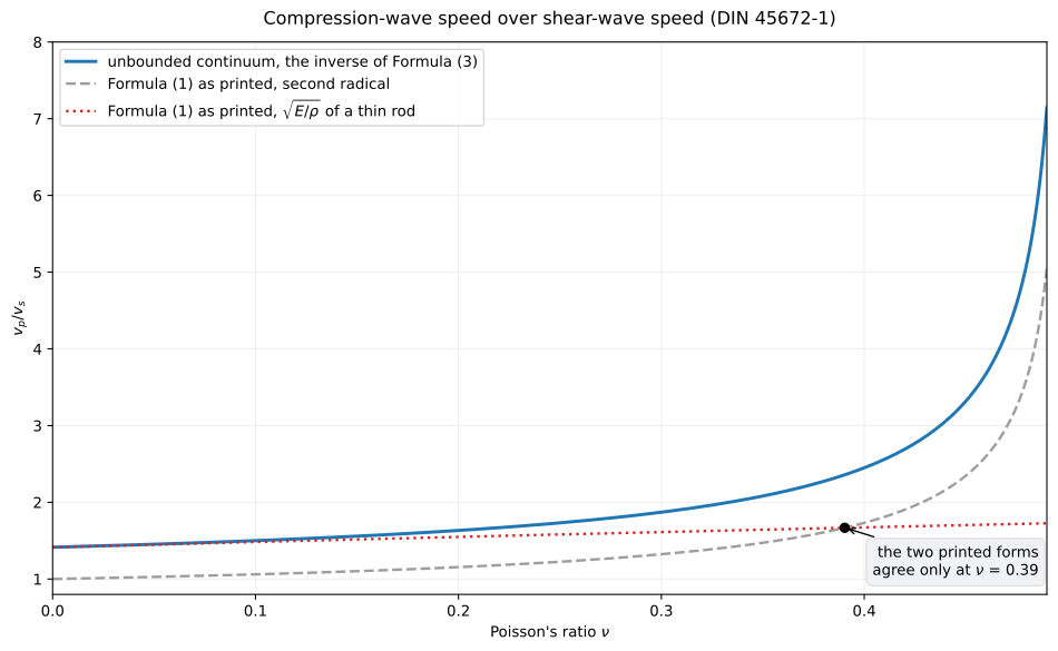
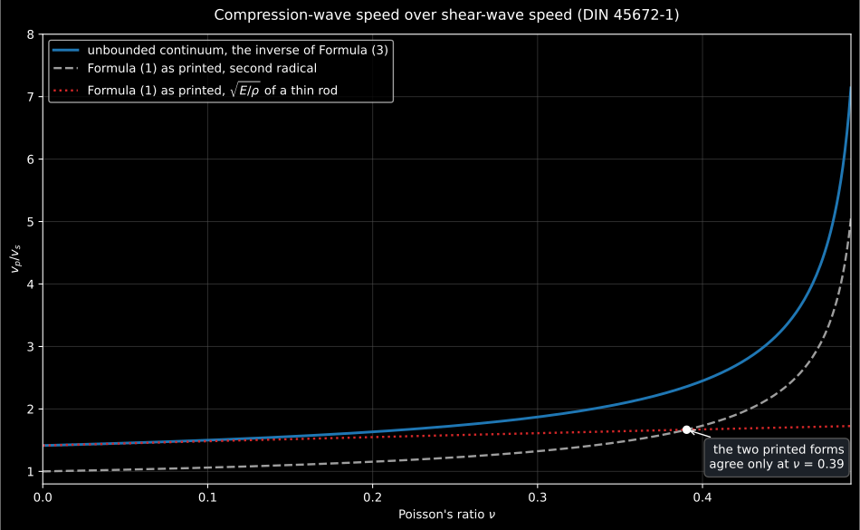
Figure code
import matplotlib.pyplot as pltimport numpy as np
from phonometry import vibration
nu = np.linspace(0.0, 0.49, 300)continuum = [    vibration.compression_wave_speed(1.0, poisson_ratio=n, density_kg_m3=1.0)    for n in nu]fig, ax = plt.subplots(figsize=(10, 6))ax.plot(nu, continuum, label="continuum, the inverse of Formula (3)")ax.plot(nu, np.sqrt((1 - nu) / (1 - 2 * nu)), "--", label="Formula (1), second radical")ax.plot(nu, np.sqrt(2 * (1 + nu)), ":", label="Formula (1), sqrt(E / rho)")ax.set_xlabel("Poisson's ratio")ax.set_ylabel("v_p / v_s")ax.legend()
The strain matters because a soil’s shear modulus falls as the strain grows:
Figure 1 of the clause has it constant up to a shear strain of about 10⁻⁴
and dropping below 20 % of that value further on. Rail traffic, and the
measurements that read the speeds, strain the ground around 10⁻⁶, so the
modulus measured is the one that applies.
8. Where the record comes from
Section titled “8. Where the record comes from”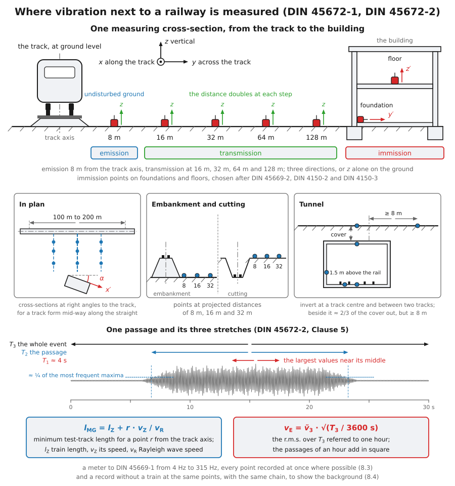
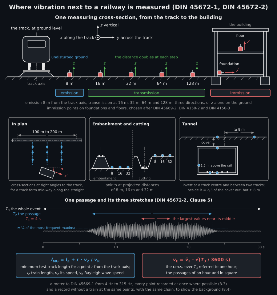
Part 1 is the other half of the pair: it says where the transducers go and what a record has to be before Part 2 may reduce it. The cross-section is 6.1, at right angles to the track, and it carries the emission point on the ground 8 m from the track axis (6.2.1.2), the transmission points at twice the distance each time out to 128 m (6.2.2), and the immission points on the building that DIN 45669-2, DIN 4150-2 and DIN 4150-3 place (6.2.3). On the ground the directions are the x, y and z of 6.4.1; in the building they are turned about z so that x′ runs along the outer wall nearest the track axis, and the normal to the room boundary is the one to prefer (6.4.4).
How the measurement goes
Section titled “How the measurement goes”Take a meter to DIN 45669-1, re-verified at least every three years and working
from 4 Hz to 315 Hz, or to 80 Hz when the result is for DIN 4150-2, and check it
after every set-up. Lay out a cross-section at right angles to the track: an
emission point on the ground 8 m from the track axis, in undisturbed ground
where possible, transmission points at 16 m, 32 m, 64 m and 128 m, and immission
points where DIN 45669-2, DIN 4150-2 and DIN 4150-3 put them. On an embankment
or in a cutting the distances are projected; beside a bridge they run from the
track axis projected on the ground next to a pier, 8 m out, or 16 m or 32 m
where the fill is large; in a tunnel the points go on the invert by preference,
at least 2 m from any joint. Measure three directions, or z alone on the
ground when fewer will do, and more than one cross-section for a stretch of
line. On rail and tunnel, glue flat metal plates with a hard insulating
adhesive; on the ground and in the building, couple as DIN 45669-2 says, and
keep the added mass within a tenth of the dynamic mass of what it measures.
Record several passages of each kind of train, every point at once where
possible, with the speed, where it matters, determined to within 5 %, and leave
out trains that brake, accelerate or meet another unless that is typical of the
site. Record the background too: same points, same chain, no train. The report
gives positions, directions, track, ground and building, and the evaluation to
DIN 45672-2.
9. What this page is not
Section titled “9. What this page is not”DIN 45672-1 is a measuring method: measurement points on the way from the track to the building, directions, coupling, the trains to record and the report to write. None of that is arithmetic and the library computes none of it, but that procedure is what decides what a record is worth, so it is set out above; the coupling it points to is DIN 45669-2. Nor is any assessment: the numbers this page produces are compared with something only in DIN 4150-2 and DIN 4150-3.
The three stretches of Clause 5, the running r.m.s. and the velocity and acceleration levels of Formulae (1) to (3), the interval r.m.s. of Formulae (4) and (5), and the event value, its level and its sum over the passages of an hour, Formulae (8) to (10).
The third-octave levels of Formulae (6) and (7) from 4 Hz to 315 Hz, or to 80 Hz as DIN 45672-1 allows, and the amplitude distribution of Formula (11).
The narrow-band densities of Formulae (12) to (14) at the resolution of 7.3.2, the conversion to third octaves of Formula (23) with every count of Table 1, the density level of Figure 7, the dimension conversion of Annex A, the quantities of Annex B and the energy averaging of Clause 9.
The ground constants of DIN 45672-1 Clause 4.5 from two wave speeds and a density, with Formulae (1) and (5) in the form the continuum gives and the printed forms registered as errata.
Not covered
No analyser. The calibration checks of 7.3.3 test the amplitude display of a narrow-band analyser, with and without a Hanning window; the library’s density is correct by construction and has nothing to calibrate.
No measuring procedure is checked, and no verdict. The measurement points, directions, coupling and choice of trains of DIN 45672-1 and DIN 45669-2 are summarised above, but nothing here checks them; what the numbers mean for people and buildings is DIN 4150-2 and DIN 4150-3.
What this guide covers
Section titled “What this guide covers”References
Section titled “References”- Deutsches Institut für Normung. (1995). Schwingungsmessungen in der Umgebung von Schienenverkehrswegen — Teil 2: Auswerteverfahren (DIN 45672-2:1995-07). The three stretches of Clause 5, the running r.m.s. and levels of Formulae (1) to (3), the interval r.m.s. of Formulae (4) and (5), the third-octave levels of Formulae (6) and (7), the event value and level of Formulae (8) to (10), the amplitude distribution of Formula (11), the power and energy spectral densities of Formulae (12) to (14) with the parameters of 7.3.2, the narrow-band to third-octave conversion of Formula (23) with Table 1, the dimension conversion of Annex A, the quantities of Annex B and the averaging over passages of Clause 9. The analyser calibration checks of 7.3.3 are not implemented.
- Deutsches Institut für Normung. (2009). Schwingungsmessungen in der Umgebung von Schienenverkehrswegen — Teil 1: Messverfahren (DIN 45672-1:2009-12). Clause 4.5: the wave speeds of Formulae (1) and (2), Poisson's ratio of Formula (3), the shear strain of Formula (4) and the moduli of Formula (5), with Formulae (1) and (5) in the corrected form registered in the errata. The measuring procedure of the rest of the standard is not arithmetic and is not implemented; the measuring conditions of Clause 6, the operating states of Clause 7, the execution of Clause 8 and the report of Clause 10 are set out in the measurement section.
- Deutsches Institut für Normung. (2010). Messung von Schwingungsimmissionen — Teil 1: Schwingungsmesser — Anforderungen und Prüfungen (DIN 45669-1:2010-09). The meter a railway measurement is made with, in its 4 Hz to 315 Hz working range, whose band limitation every quantity here is read after.