Human Vibration

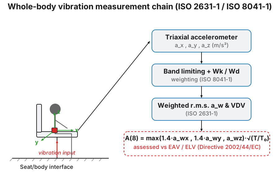
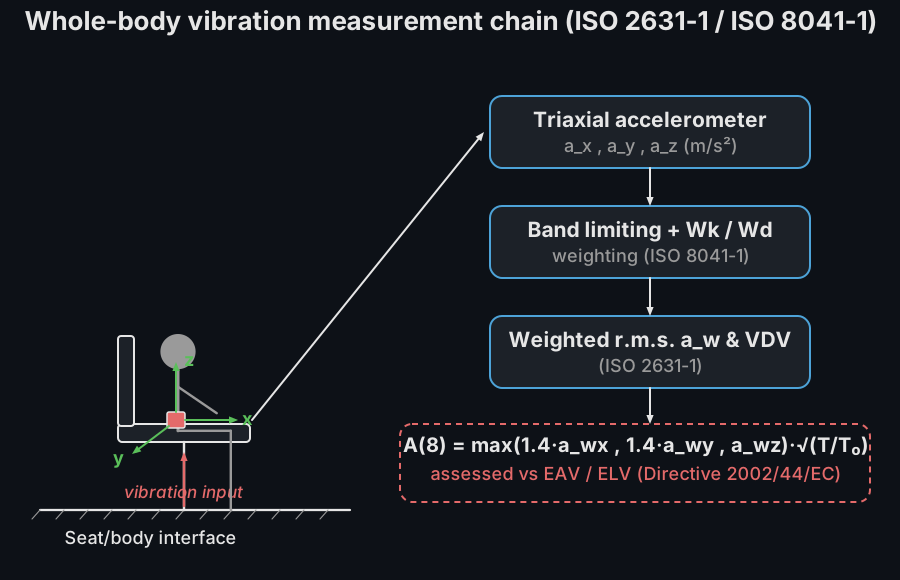
Vibration transmitted to a person is evaluated with the same measurement chain whatever its origin: the acceleration is frequency-weighted to reflect how the body responds at each frequency, reduced to a weighted r.m.s. acceleration (with dose measures for shocks and long records), condensed across axes into a single magnitude (the vibration total value for hand-arm exposure and for comfort; the highest axis value for the whole-body health assessment), and finally normalised to an 8-hour daily exposure $A(8)$ that is compared against the action and limit values of the European directive.

The weightings themselves are defined once, in ISO 8041-1:2017, as a cascade of analog filters; ISO 2631-1 applies them to whole-body vibration, ISO 2631-2 to vibration in buildings, ISO 2631-4 to rail ride comfort, and ISO 5349-1/-2 to hand-transmitted vibration. This page covers the whole chain.

0. Getting the numbers

Every magnitude on this page is a measured one, and the two halves of the subject are instrumented differently: the whole-body chain measures the surface a person sits, stands or lies on, the hand-arm chain measures the handle of a tool while it is being used.

Whole body: at the interface, and nowhere else (ISO 2631-1, 5.2–5.3)

The transducer goes where the vibration enters the body, on the surface between the body and that surface (5.3.1). For a seated person that means three principal contact areas: the seat surface beneath the ischial tuberosities, the seat back at the principal area of support, and the feet on the surface they rest on; for a recumbent person, under the pelvis, the back and the head. A rigid surface may be measured close to the contact area instead, usually within 10 cm of its centre; a seat back that cannot be reached may be measured on the frame behind the cushion and then corrected for the transmissibility of the cushion. Every measurement location must be reported.

On a resilient surface — a seat cushion, a couch — the transducer is interposed between the person and the surface in a suitably formed mount that does not greatly alter the pressure distribution (5.3.2); the commonly used design for that mount is the semi-rigid disc of ISO 10326-1, drawn to size on Multiple Shock Vibration. The person adopts the posture that is normal for the environment.

The three translational transducers at one location are positioned orthogonally and as close together as practicable (5.2.3). Where perfect alignment with the basicentric axes is impracticable, up to 15° of deviation is allowed, and the orientation of the axes relative to gravity is recorded (5.2.2) — on an inclined seat the z axis is not vertical. The duration of measurement must be long enough for reasonable statistical precision and typical of the exposure being assessed, and it is reported with the result (5.5).

Hand-arm: on the handle, in the gripping zone (ISO 5349-2, 6.1)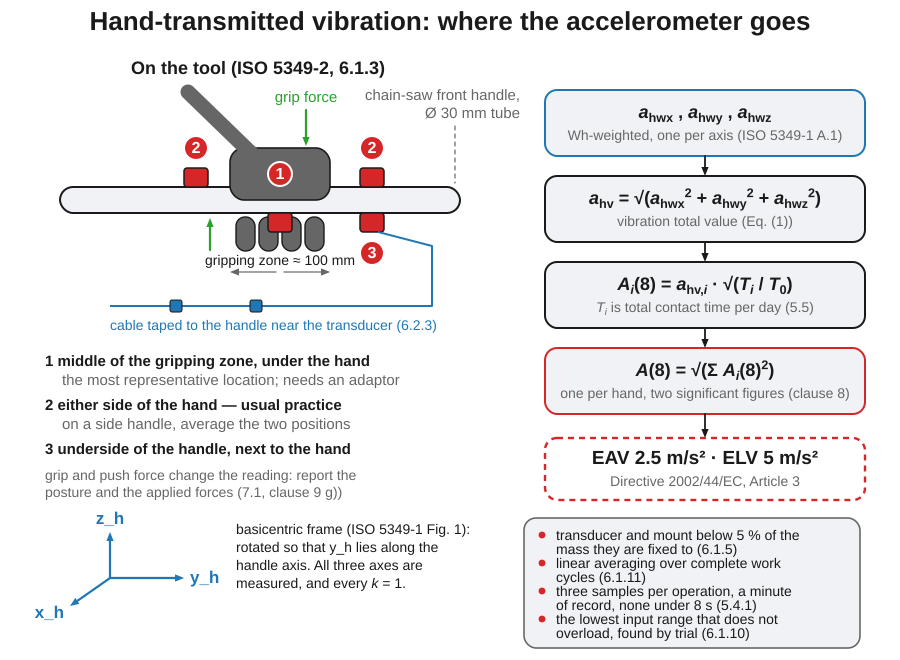

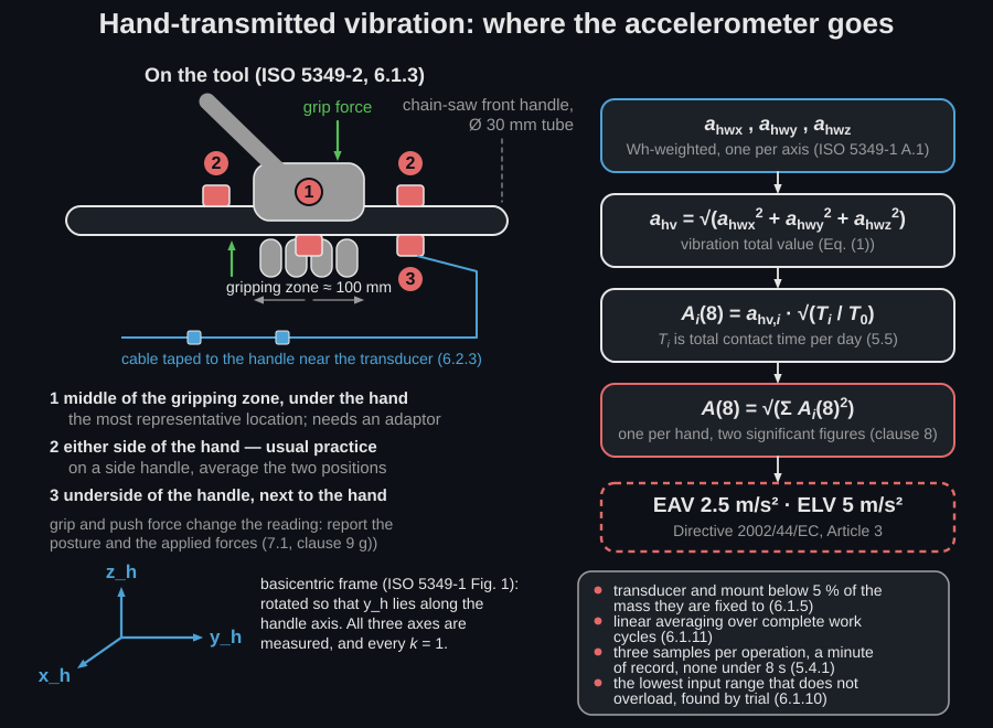
The accelerometer belongs at or near the surface of the hand where the vibration enters the body, preferably at the middle of the gripping zone — halfway along the width of the hand on the handle (6.1.3). That position usually needs a mounting adaptor that fits under the hand or between the fingers, so in practice the transducers go either side of the hand or on the underside of the handle adjacent to the middle of the hand. Where the vibration differs across the width of the hand — flexibly mounted side handles on angle grinders are the standard case — two positions either side of the hand are used and averaged. The measurement is made for each gripping zone the operator actually uses, and the locations and orientations are reported with a sketch and dimensions (clause 9).

Three constraints decide whether the mounting is acceptable:

• Mass (6.1.5). Accelerometer plus mount below 5 % of the mass of the tool, handle or workpiece it is fixed to; practical triaxial systems under 30 g have been achieved. If in doubt, repeat the measurement with an equal added mass beside the transducer: a markedly different magnitude means a lighter mount.
• Attachment (6.1.4). Rigid, flat in frequency response over the measured band, checked before and after, and not obstructing the tool’s controls. A soft handle coating is either removed under the transducer or fully compressed by the fixing; a thick resilient layer that may itself be reducing exposure needs an adaptor held in place by the operator’s own grip.
• Posture and force (7.1). Mounting a transducer changes how the tool is held and how much grip and push force is applied, and the standard lists that change among the dominant uncertainty contributions — larger, it notes, than instrumentation or calibration. The grip and feed forces belong in the report.

What the magnitude is an average of (ISO 5349-2, 5.4 and 6.1.11)

Every $a_{hv}$ fed to the exposure calculation below is an average, and the averaging rule is normative: magnitudes are averaged over periods of normal use of the tool or of contact with the workpiece, using linear averaging over one or more complete operations or work cycles (6.1.11). Exponential averaging is admitted only where the instrument cannot do linear averaging and the signal is steady enough to give a reliable average. Clause 5.4.1 fixes the sampling: at least three samples per operation, a total measuring time of at least one minute, several short samples in preference to one long one, and samples shorter than about 8 s avoided because they do not evaluate the low-frequency components reliably. Where the user selects the instrument’s input range, trial measurements set it to the lowest range that does not overload (6.1.10).

When the number is wrong (ISO 5349-2, 6.2 and 6.3)

The characteristic faults of hand-arm measurement all produce a plausible number rather than an obvious failure:

• Cable and connector faults (6.2.1), the most common problem of all. A total loss of connection reads as no vibration; an intermittent one reads as DC offsets with a normal-looking signal between them. Faulty screening lets mains frequencies in, which on an electric tool is nearly undetectable because the dominant vibration frequency is usually harmonically related to the mains.
• Electromagnetic interference (6.2.2): screened, twisted cables, the screen earthed at one end only, no runs parallel to power cables, and electrical insulation between the accelerometer and the vibrating surface.
• Triboelectric signal (6.2.3): a cable under high-amplitude vibrational stress generates charge by deformation, so it is secured to the vibrating surface close to the accelerometer — taped to the handle, or clipped along the air line on a pneumatic tool.
• DC-shift (6.2.4), the one that inflates a result rather than destroying it. Very high accelerations at high frequency — percussive tools with no damping system — mechanically overload a piezoelectric transducer and add a false low-frequency component, exactly where the weighting has most gain. It shows in a frequency analysis as unrealistically high low-frequency values, and the standard’s check is to convert the unweighted band r.m.s. acceleration to a displacement, $d=a/(40f^2)$, and compare it with the motion of the transducer you can actually see:

import numpy as np

# Unweighted one-third-octave r.m.s. acceleration on a chipping hammer,
# low-frequency bands only (m/s^2), and the displacement they imply (mm).
bands = np.array([8.0, 10.0, 12.5, 16.0, 20.0])
accel = np.array([9.0, 14.0, 6.0, 3.0, 2.0])
print((1000.0 * accel / (40.0 * bands**2)).round(2))   # [3.52 3.5  0.96 0.29 0.12]

A handle visibly moving a millimetre cannot be moving 3.5; a factor of two or more between the computed and the observed motion means DC-shift is likely. A mechanical filter is the countermeasure, and a record showing DC-shift is discarded — the distortion affects the whole spectrum, so deleting the low-frequency bands does not rescue it.

Finally, the chain is checked with a vibration calibrator before and after every sequence of measurements (6.3.1), and the whole system is verified against the ISO 8041 tolerances on a regular basis, typically every two years and always after rough handling; the results of those verification checks are recorded (6.3.2). That record is what the fiche’s calibration field of section 5 exists to carry.

1. Frequency weightings (ISO 8041-1)

Every human-vibration weighting is the product of four analog stages evaluated at $s=j2\pi f$ (ISO 8041-1 Formulae (1)–(5)): a second-order Butterworth high-pass and low-pass band limiting, an acceleration–velocity transition carrying the overall gain $K$, and an upward step:

$$H(s)=H_h(s)H_l(s)H_t(s)H_s(s).$$

A single Table 3 parameter set $(f_1,Q_1,f_2,Q_2,f_3,f_4,Q_4,f_5,Q_5,f_6,Q_6,K)$ realises all nine weightings (Wb, Wc, Wd, We, Wf, Wh, Wj, Wk, Wm), with a corner set to infinity collapsing its stage to unity. The principal whole-body weighting is Wk (vertical, seat surface); Wd is the horizontal weighting, and Wh the hand-arm weighting.

from phonometry import vibration

# The overall weighting response at any frequencies (ISO 8041-1 Formula (5)).
# 6.3096 Hz is the *true* centre of the nominal 6.3 Hz band, which is where
# the Annex B tables print their factors.
resp = vibration.frequency_weighting("Wk", [1.0, 6.3096, 20.0])
print(resp.magnitude.round(3))      # [0.482 1.054 0.636]  (factors)
print(resp.magnitude_db.round(2))   # [-6.33  0.46 -3.93]  (dB)

The factors reproduce the ISO 8041-1 Annex B design-goal tables to their four significant figures: Wk plateaus near −6 dB below 2 Hz, peaks at +0.46 dB near 6.3 Hz and rolls off above.

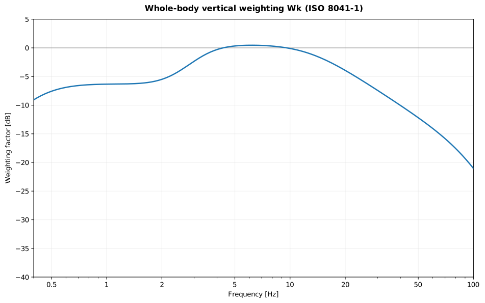
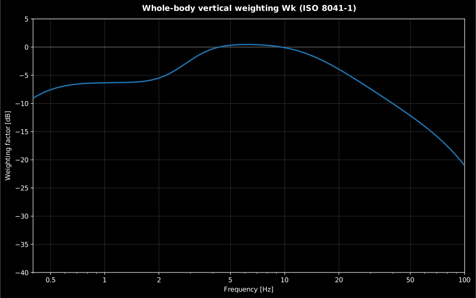
The one feature to read is the small peak just above 6 Hz: that is the vertical whole-body resonance of a seated person, and it is the reason the weighting exists. Everything else is the band limiting on either side of it.

Show the code for this figure

import numpy as np
import matplotlib.pyplot as plt
from phonometry import vibration

result = vibration.frequency_weighting("Wk", np.geomspace(0.4, 100.0, 240))

# One line:
result.plot()
plt.show()

# By hand, from the result's fields, mirroring what WeightingResponse.plot() draws:
fig, ax = plt.subplots()
ax.semilogx(result.frequencies, result.magnitude_db, color="#1f77b4")
ax.set_xlabel("Frequency [Hz]")
ax.set_ylabel("Weighting factor [dB]")
ax.set_title("Whole-body vertical weighting Wk (ISO 8041-1)")
plt.show()

To weight a time signal, apply_weighting applies the exact complex response in the frequency domain (so magnitude and phase match the standard), which the time-domain dose metrics below then consume.

Which weighting on which axis

The weighting is selected by posture, measurement point and axis, not by application alone. ISO 2631-1 (Tables 1 and 2, clauses 7.2.3 and 8.2.2) maps them as follows; the multiplying factors $k$ return in the vibration total value of section 3:

Posture, measurement point	Axis	Weighting	$k$ health	$k$ comfort
Seated, seat surface	x, y	Wd	1.4	1.0
Seated, seat surface	z	Wk	1.0	1.0
Seated, seat surface (rotation)	rx / ry / rz	We	—	0.63 / 0.40 / 0.20 m/rad
Seated, backrest	x	Wc	(0.8)¹	0.8
Seated, backrest	y / z	Wd	—	0.5 / 0.4
Seated, feet	x / y / z	Wk	—	0.25 / 0.25 / 0.4
Standing, floor	x, y	Wd	—	1.0
Standing, floor	z	Wk	—	1.0
Recumbent, under the pelvis	horizontal	Wd	—	1.0
Recumbent, under the pelvis	vertical	Wk	—	1.0
Recumbent, under the head	vertical	Wj	—	1.0
Motion sickness (clause 9)	vertical	Wf	—	—

¹ The health assessment of clause 7 is defined on the seat surface; the backrest x measurement with Wc, $k=0.8$ is encouraged but excluded from the Annex B severity assessment (7.2.3).

The remaining three weightings belong to the companion parts rather than to ISO 2631-1’s posture map: Wm for building occupants on all axes (ISO 2631-2), Wb for vertical rail ride comfort (ISO 2631-4), and Wh for hand-transmitted vibration on all three hand axes with every $k=1$ (ISO 5349-1) — which is why the hand-arm total of section 3 is a plain vector sum with no multiplying factors in it.

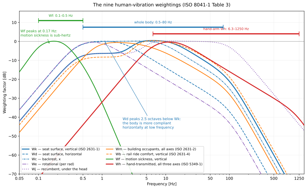
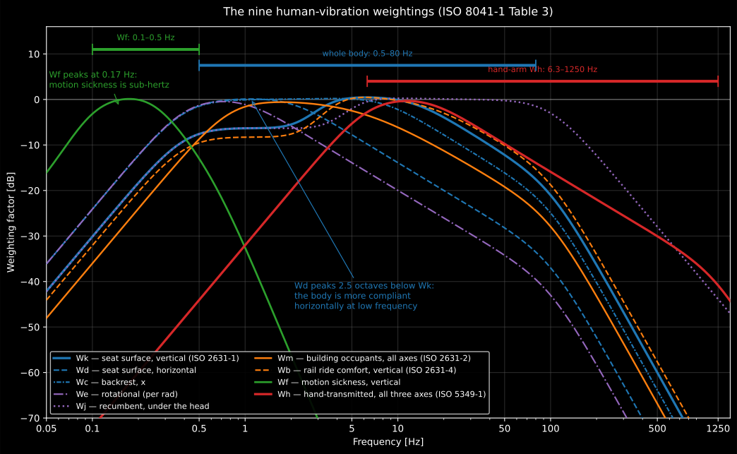
Three families on one axis. Wf peaks at 0.17 Hz because motion sickness is a sub-hertz phenomenon; the whole-body weightings peak between 1 and 6 Hz, Wd two and a half octaves below Wk because the body is far more compliant horizontally at low frequency; and Wh is still 37 dB down at 1 kHz where Wk is 78 dB down, because the hand follows tool frequencies the torso cannot. The bars above the curves are the bands the ISO tables cover: 0.1–0.5 Hz for Wf, 0.5–80 Hz for the whole-body set (band-limited at 0.4 and 100 Hz, ISO 2631-1 6.4.1.1) and 6.3–1250 Hz for Wh (band-limited at 6.31 and 1258.9 Hz, ISO 5349-1 Table A.1).

Show the code for this figure

import numpy as np
import matplotlib.pyplot as plt
# `vibration` is the namespace imported in the snippet of section 1.

freqs = np.geomspace(0.05, 1500.0, 900)

fig, ax = plt.subplots(figsize=(11, 6.8))
for name in vibration.WEIGHTING_NAMES:
    factors = np.asarray(vibration.weighting_factors(name, freqs))
    ax.semilogx(freqs, 20.0 * np.log10(np.maximum(factors, 1e-9)), label=name)
ax.set_xlabel("Frequency [Hz]")
ax.set_ylabel("Weighting factor [dB]")
ax.set_xlim(0.05, 1500.0)
ax.set_ylim(-70.0, 16.0)
ax.legend(loc="lower left", ncol=2, fontsize=8.5)
plt.show()

2. Weighted acceleration and dose measures (ISO 2631-1)

The basic evaluation is the weighted r.m.s. acceleration. From a one-third-octave spectrum it is (ISO 2631-1 Eq. (9); the identical construction gives the hand-arm $a_{hw}$ of ISO 5349-1 Eq. (A.1)):

$$a_w=\sqrt{\sum _i{\left(W_i{a}_i\right)}^2},$$

with $W_i$ the weighting factor at band centre $i$ and $a_i$ the measured band acceleration. The factors are evaluated at exactly the frequencies you pass; note that the ISO tables (ISO 8041-1 Annex B, ISO 2631-1 Table 3, ISO 5349-1 Table A.2) tabulate $W_i$ at the true one-third-octave centres $10^{n/10}$ Hz (6.31, 7.943, 15.85, …), not at the nominal band labels (6.3, 8, 16, …); pass true centres when comparing against the tabulated factors.

import numpy as np
from phonometry import vibration

# A measured vertical seat spectrum (r.m.s. per one-third octave, m/s^2),
# the same 19 bands the figure below is drawn from.
freqs = np.array([1.0, 1.25, 1.6, 2.0, 2.5, 3.15, 4.0, 5.0, 6.3, 8.0, 10.0,
                  12.5, 16.0, 20.0, 25.0, 31.5, 40.0, 63.0, 80.0])
accel = np.array([0.18, 0.24, 0.33, 0.46, 0.52, 0.55, 0.48, 0.39, 0.31, 0.26,
                  0.21, 0.17, 0.13, 0.10, 0.078, 0.060, 0.045, 0.028, 0.020])

result = vibration.weighted_acceleration(accel, freqs, "Wk")
print(round(result.overall, 3))          # 1.026  m/s^2 (a_w)
print(result.weighted.round(3))          # W_i * a_i per band

# The W_i themselves, at the true centres of the nominal 6.3 and 16 Hz bands:
# these are the numbers the ISO tables print, and what the sum multiplies by.
print(vibration.weighting_factors("Wk", [6.3096, 15.849]).round(3))   # [1.054 0.774]

result.plot()   # unweighted vs weighted bands, as in the figure below (needs matplotlib)

Those band labels are the nominal ones, for legibility. Passing the true centres $10^{n/10}$ Hz (1, 1.259, 1.585, … 79.433) instead moves $a_w$ from 1.0260 to 1.0267 m/s², so the caution above is about comparing a single $W_i$ against a printed table, not about a broadband r.m.s., where the two agree to three figures.

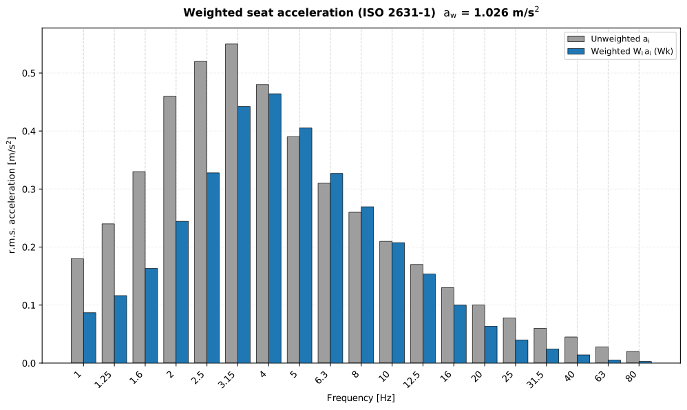
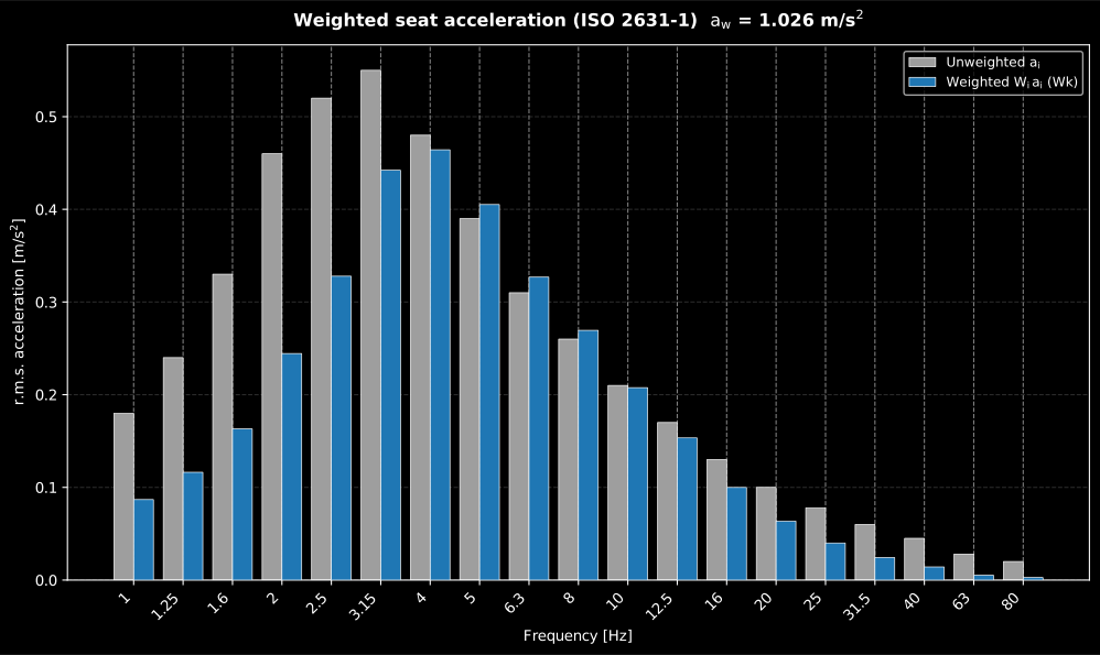
The weighting leaves the 4–8 Hz bands almost untouched and throws away everything above 20 Hz, so $a_w$ = 1.026 m/s² is set by three bands out of nineteen. A vehicle seat is judged on the part of its spectrum it was least able to isolate.

Show the code for this figure

import numpy as np
import matplotlib.pyplot as plt
from phonometry import vibration

freqs = np.array([1.0, 1.25, 1.6, 2.0, 2.5, 3.15, 4.0, 5.0, 6.3, 8.0, 10.0,
                  12.5, 16.0, 20.0, 25.0, 31.5, 40.0, 63.0, 80.0])
accel = np.array([0.18, 0.24, 0.33, 0.46, 0.52, 0.55, 0.48, 0.39, 0.31, 0.26,
                  0.21, 0.17, 0.13, 0.10, 0.078, 0.060, 0.045, 0.028, 0.020])
result = vibration.weighted_acceleration(accel, freqs, "Wk")

# One line:
result.plot()
plt.show()

# By hand, mirroring what WeightedSpectrum.plot() draws:
pos = np.arange(freqs.size)
fig, ax = plt.subplots()
ax.bar(pos - 0.2, result.band_accelerations, 0.4, color="#bbbbbb",
       label="Unweighted $a_i$")
ax.bar(pos + 0.2, result.weighted, 0.4, color="#1f77b4",
       label="Weighted $W_i a_i$ (Wk)")
ax.set_xticks(pos)
ax.set_xticklabels([f"{f:g}" for f in freqs], rotation=45, ha="right")
ax.set_xlabel("Frequency [Hz]")
ax.set_ylabel("r.m.s. acceleration [m/s²]")
ax.set_title(f"Weighted acceleration ($a_w$ = {result.overall:.3f} m/s²)")
ax.legend()
plt.show()

When the r.m.s. value understates an intermittent or shock-laden exposure, ISO 2631-1 adds dose measures computed on the weighted time signal: the running r.m.s. $a_w(t_0)$ (Eqs. (2)/(3)) and its maximum, the maximum transient vibration value MTVV (Eq. (4), the maximum of the running r.m.s. with a 1 s integration time); the fourth-power vibration dose value $\text{VDV}={\left(\int a_w^{4}dt\right)}^{1/4}$ (Eq. (5)); the motion sickness dose value $\text{MSDV}={\left(\int a_w^{2}dt\right)}^{1/2}$ (Annex D, on the Wf-weighted vertical axis, not Wk); and the crest factor (peak / r.m.s.), whose value above 9 signals that the basic method is inadequate.

Deciding whether the basic method is enough (clause 6.3.3)

The crest factor is the weaker of the two available tests, and the standard says so twice: clause 6.2.2 notes that the basic method may underestimate severity even when the crest factor is not greater than 9, and the notes to Annexes B and C call it “an uncertain method” of deciding whether the r.m.s. may be used. The criteria that actually decide are two ratios, and either one exceeded means the additional method matters for the judgement:

$$\frac{\text{MTVV}}{a_w}=1,5,\frac{\text{VDV}}{a_w{T}^{1/4}}=1,75.$$

$\text{MTVV}/a_w$ asks whether any single second of the record is much worse than the record as a whole; $\text{VDV}/(a_w{T}^{1/4})$ asks whether the fourth power finds peaks that the second power averaged away. Whichever is used, clause 6.1 requires both the basic value and the additional value to be reported, and clause 5.6 adds the measurement period of the crest factor.

Gaussian noise is the case in which nothing goes wrong, and computing the two ratios for it is how you learn to read them:

import numpy as np
from phonometry import vibration

fs = 1000.0
duration = 60.0
raw = np.random.default_rng(0).standard_normal(int(duration * fs))   # 60 s record
a_w = vibration.apply_weighting(raw, fs, "Wk")                       # weighted signal
rms = float(np.sqrt(np.mean(np.asarray(a_w) ** 2)))

vdv = vibration.vibration_dose_value(a_w, fs)
mtvv = vibration.mtvv(a_w, fs)
print(round(rms, 3), round(vdv, 3), round(mtvv, 3))   # 0.204  0.744  0.265
print(round(vibration.crest_factor(a_w), 2))          # 3.74   crest factor
print(round(mtvv / rms, 2))                           # 1.3   < 1.5
print(round(vdv / (rms * duration**0.25), 2))         # 1.31  < 1.75

# running_rms returns the whole a_w(t_0) series MTVV is only the maximum of:
# it is what you plot to find *where* in a shift the transient happened.
running = vibration.running_rms(a_w, fs, integration_time=1.0)
print(round(float(np.max(running)), 3))               # 0.265, the MTVV above

Every criterion passes, which is the point: the example proves the rule is not being triggered, not that the exposure is severe. A record with shocks in it behaves differently — five impacts on a 4.5 Hz ride oscillation, the ordinary content of an off-road seat:

fs_shock, duration_shock = 200.0, 20.0
time = np.arange(int(duration_shock * fs_shock)) / fs_shock
rng = np.random.default_rng(3)
seat = 0.35 * np.sin(2 * np.pi * 4.5 * time) + 0.10 * rng.standard_normal(time.size)
for start, amplitude in ((2.6, 9.0), (6.1, 14.0), (9.4, 6.0), (13.8, 18.0), (17.2, 11.0)):
    hit = time >= start
    seat[hit] += amplitude * np.exp(-28.0 * (time[hit] - start)) * np.sin(
        2 * np.pi * 8.0 * (time[hit] - start))

a_ws = np.asarray(vibration.apply_weighting(seat, fs_shock, "Wk"))
rms_s = float(np.sqrt(np.mean(a_ws**2)))
mtvv_s = vibration.mtvv(a_ws, fs_shock)
vdv_s = vibration.vibration_dose_value(a_ws, fs_shock)
print(round(rms_s, 3), round(mtvv_s, 3), round(vdv_s, 3))   # 0.529  1.432  3.011
print(round(vibration.crest_factor(a_ws), 2))               # 13.49  > 9
print(round(mtvv_s / rms_s, 2))                             # 2.71   > 1.5
print(round(vdv_s / (rms_s * duration_shock**0.25), 2))     # 2.69   > 1.75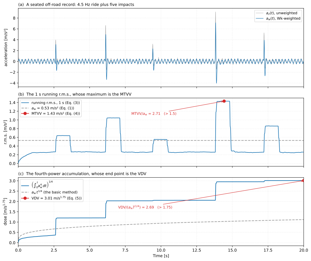

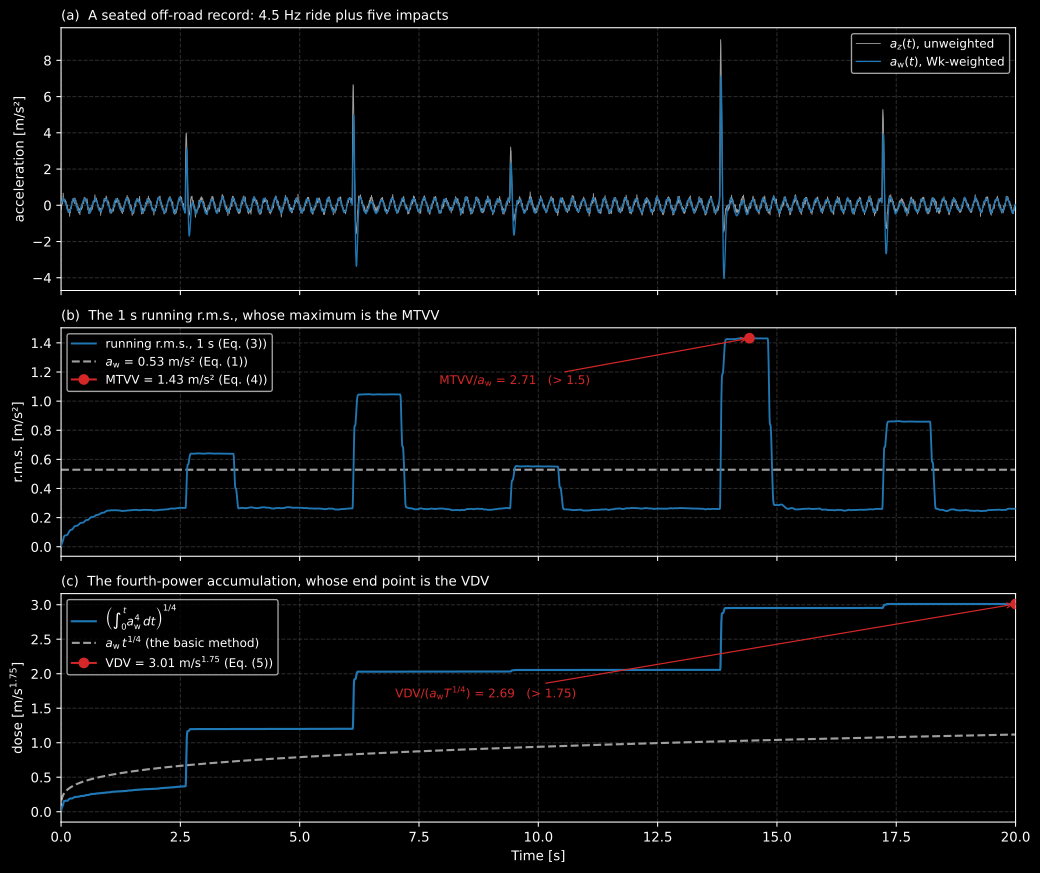
The same twenty seconds judged three ways. The r.m.s. barely notices the five impacts, the running r.m.s. finds them one at a time, and the fourth-power accumulation climbs in a step at each of them — which is why the two ratios of clause 6.3.3 are 2.71 and 2.69 here and 1.3 and 1.31 on the Gaussian record above. Any of the three criteria would have sent this record to the additional methods; the crest factor is simply the one that catches it last.

Show the code for this figure

import numpy as np
import matplotlib.pyplot as plt

# `seat`, `a_ws`, `rms_s`, `fs_shock` and `time` come from the snippet above.
running = np.asarray(vibration.running_rms(a_ws, fs_shock, integration_time=1.0))
fourth = (np.cumsum(a_ws**4) / fs_shock) ** 0.25

fig, (ax_t, ax_r, ax_v) = plt.subplots(3, 1, sharex=True, figsize=(11, 9.2))
ax_t.plot(time, seat, lw=0.7, color="#9e9e9e", label="$a_z(t)$, unweighted")
ax_t.plot(time, a_ws, lw=1.0, color="#1f77b4",
          label=r"$a_\mathrm{w}(t)$, Wk-weighted")
ax_r.plot(time, running, lw=1.4, color="#1f77b4", label="running r.m.s., 1 s")
ax_r.axhline(rms_s, ls="--", color="#9e9e9e", label=rf"$a_\mathrm{{w}}$ = {rms_s:.2f}")
ax_v.plot(time, fourth, lw=1.6, color="#1f77b4",
          label=r"$(\int a_\mathrm{w}^4)^{1/4}$")
ax_v.plot(time, rms_s * time**0.25, ls="--", color="#9e9e9e",
          label=r"$a_\mathrm{w} t^{1/4}$")
for axis in (ax_t, ax_r, ax_v):
    axis.legend(loc="upper left", fontsize=9)
ax_v.set_xlabel("Time [s]")
plt.show()

Motion sickness: the one dose measure with a published reading

MSDV is the only measure on this page that converts directly into an expected number of people. It is computed on the Wf-weighted z-axis acceleration over the whole period during which motion could occur (Annex D, method (a)); for a continuous motion of roughly constant magnitude it may instead be estimated from a short-period r.m.s. as ${\text{MSDV}}_z=a_w{T}_0^{1/2}$ (method (b)), whose measurement period should not normally be less than 240 s. The reading is that the percentage of people who may vomit is approximately $K_m{\text{MSDV}}_z$, with $K_m=1/3$ for a mixed population of unadapted male and female adults, over exposures from about 20 min to about 6 h and prevalences up to about 70 %; the estimate can be exceeded when $a_w$ is above 0.5 m/s². Females are more prone than males, and prevalence declines with age.

# A 240 s sample of ship heave at 0.2 Hz, the band Wf is built for.
fs_ms = 20.0
t_ms = np.arange(int(240 * fs_ms)) / fs_ms
heave = 0.45 * np.sin(2 * np.pi * 0.2 * t_ms)
a_wf = np.asarray(vibration.apply_weighting(heave, fs_ms, "Wf"))

msdv = vibration.motion_sickness_dose_value(a_wf, fs_ms)
print(round(msdv, 1), round(msdv / 3.0, 1))    # 4.9 m/s^1.5 -> 1.6 % over 240 s

# Method (b): the same magnitude sustained for a four-hour crossing.
sustained = float(np.sqrt(np.mean(a_wf**2))) * (4 * 3600.0) ** 0.5
print(round(sustained, 1), round(sustained / 3.0, 1))   # 37.9 -> 12.6 %

Note the weighting: an MSDV computed from the Wk-weighted signal used everywhere else on this page would be meaningless, because Wk is 18.3 dB down at 0.2 Hz where Wf is 0.1 dB down.

3. Vibration total value and daily exposure A(8)

Across the three axes the vibration total value combines the axis-weighted r.m.s. accelerations with the posture multiplying factors $k_j$ (ISO 2631-1 Eq. (10); for hand-arm, ISO 5349-1 Eq. (1) with every $k=1$):

$$a_v=\sqrt{\sum _j{k}_j^2{a}_{wj}^2}.$$

from phonometry import vibration

# Health, seated: k = 1.4 / 1.4 / 1.0 (ISO 2631-1, 7.2.3).
a_v = vibration.vibration_total_value([0.35, 0.28, 0.62], k=[1.4, 1.4, 1.0])
print(round(a_v, 3))     # 0.882  m/s^2

Health or comfort? Two different readings of the same measurement. The health assessment of clause 7 stays per axis: each axis-weighted r.m.s. (with $k$ = 1.4 / 1.4 / 1.0 seated) is judged by the highest single axis value against the Annex B health guidance caution zone, a band based mainly on 4 h to 8 h exposures below which health effects are not clearly documented, inside which caution is indicated and above which risks are likely; Directive 2002/44/EC turns that guidance into the enforceable $A(8)$ action and limit values used below. The comfort assessment of clause 8 instead combines all axes (and, where relevant, backrest, feet and rotation) into the vibration total value $a_v$ with its own $k$ set and reads it on the Annex C scale for public transport.

Overall vibration total value $a_v$	Likely reaction
less than 0.315 m/s²	not uncomfortable
0.315 m/s² to 0.63 m/s²	a little uncomfortable
0.5 m/s² to 1 m/s²	fairly uncomfortable
0.8 m/s² to 1.6 m/s²	uncomfortable
1.25 m/s² to 2.5 m/s²	very uncomfortable
greater than 2 m/s²	extremely uncomfortable

The bands overlap on purpose, and the overlap is the whole message: 0.5 m/s² is simultaneously “a little uncomfortable” and “fairly uncomfortable”, because the scale describes a distribution of reactions rather than a classification. That is also why ISO 2631-1 defines no comfort limit — acceptable magnitudes depend on trip duration and on what the passengers are trying to do (reading, eating, writing), on noise and on temperature. Quote the band, not a verdict. For orientation at the other end of the scale, the median perception threshold of a Wk-weighted vibration is about 0.015 m/s² peak, with an interquartile range from about 0.01 to 0.02 m/s² (Annex C.3).

Vibration in buildings (ISO 2631-2)

Building vibration is a third reading of the same measurement, and it breaks the “which weighting on which axis” table above. ISO 2631-2:2003 recommends the combined weighting Wm irrespective of the measurement direction (4.4); the ISO 2631-1 weightings may be used instead only where the occupant’s posture is defined. The evaluation identifies the axis with the highest frequency-weighted magnitude and uses that direction (4.5.1), and unweighted time histories over 1 Hz to 80 Hz should be recorded so that a future re-evaluation remains possible. Sources are categorised as continuous or semi-continuous (industry), permanent intermittent (traffic) or of limited duration (construction), because different magnitudes may be acceptable for each (4.5.2).

What the 2003 edition deliberately does not give is a set of acceptable magnitudes: clause 1 states that they are not given, and the Foreword records that the guidance values of the 1989 edition were dropped because their possible range is too widespread to be reproduced in an International Standard. A reader who goes looking for a building limit in ISO 2631-2 will not find one. What clause 5 gives instead is the number that matters in practice: adverse comment in residential situations arises when magnitudes are only slightly above the perception threshold — the 0.015 m/s² above — and complaints often come from the secondary effect of re-radiated noise rather than from the motion itself.

The daily exposure normalises the exposure magnitude $a$ to a reference 8-hour day ($T_0=28800$ s). For a single operation $A(8)=a\sqrt{T/T_0}$; several operations combine through their partial exposures $A_i(8)=a_i\sqrt{T_i/T_0}$ as $A(8)=\sqrt{{\sum }_i{A}_i(8{)}^2}$ (ISO 5349-1 Eqs. (2)/(3); ISO 5349-2 Eqs. (1)–(3)). Directive 2002/44/EC fixes which magnitude $a$ each kind is based on (Annex, points 1): for hand-arm vibration the vector total $a_{hv}$ (Part A), but for whole-body vibration the highest frequency-weighted axis value $\max (1.4a_{wx},1.4a_{wy},a_{wz})$ (Part B), not the vector total $a_v$ above. wbv_exposure_basis returns that dominant-axis value:

from phonometry import vibration

# Directive 2002/44/EC whole-body basis (Annex Part B): the dominant axis.
a = vibration.wbv_exposure_basis(0.35, 0.28, 0.62)
print(round(a, 3))    # 0.62  m/s^2 (max of 0.49, 0.392, 0.62; not a_v = 0.882)

daily_vibration_exposure builds the partial exposures, combines them and assesses the result against Directive 2002/44/EC: hand-arm action value $A(8)=2.5$ and limit value 5 m/s²; whole-body action 0.5 and limit 1.15 m/s² (or a VDV of 9.1 / 21 m/s¹·⁷⁵):

from phonometry import vibration

# ISO 5349-2 Annex E.3: a forestry worker's three chain-saw tasks. The times
# are *contact* times: 2 h of continuous brush-saw work, then 30 trees felled
# at 2 min each (1 h) and stripped at 4 min each (2 h).
result = vibration.daily_vibration_exposure(
    total_values=[4.6, 6.0, 3.6],                 # a_hv per task, m/s^2
    durations_s=[2 * 3600, 1 * 3600, 2 * 3600],   # total contact time per day
    kind="hav",
    labels=["brush-saw", "felling", "stripping"],
)
print(result.partials.round(2))            # [2.3  2.12 1.8 ]  A_i(8)
print(round(result.a8, 2))                 # 3.61  m/s^2 (report it as 3.6)
print(result.assessment.zone)             # 'action'  (2.5 <= A(8) < 5.0)

result.plot()   # partial exposures and A(8) against the EAV/ELV, as in the figure below (needs matplotlib)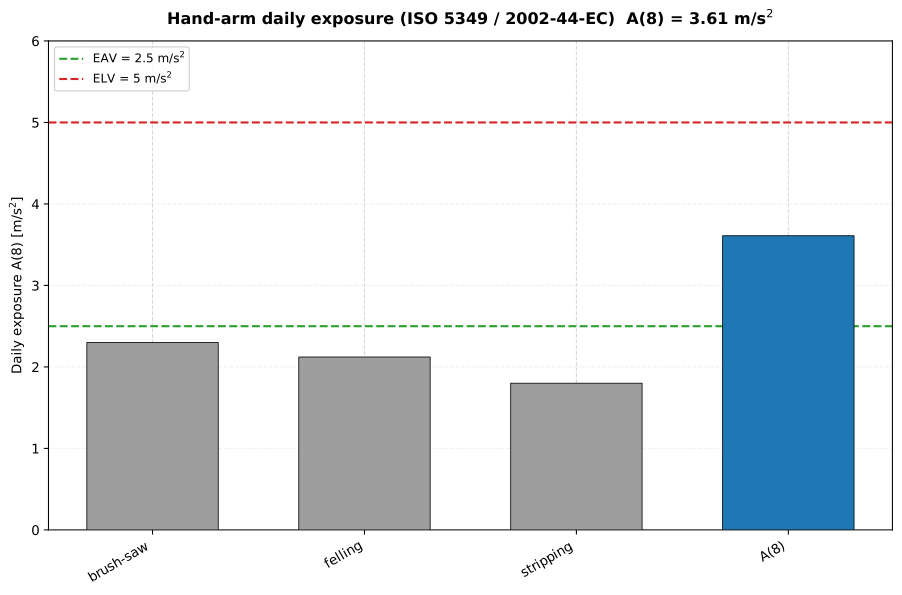

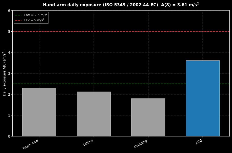
The shortest task is not the smallest contributor. Felling runs for one hour against two for the brush-saw, and still lands within 8 % of it, because $A_i(8)$ goes as $\sqrt{T_i}$ while it goes as $a_{hv}$ directly: halving the time costs 29 %, raising the magnitude from 4.6 to 6.0 m/s² buys 30 %.

Show the code for this figure

import numpy as np
import matplotlib.pyplot as plt
from phonometry import vibration

result = vibration.daily_vibration_exposure(
    [4.6, 6.0, 3.6], [2 * 3600, 1 * 3600, 2 * 3600], kind="hav",
    labels=["brush-saw", "felling", "stripping"],
)

# One line:
result.plot()
plt.show()

# By hand, mirroring what DailyVibrationExposure.plot() draws:
labels = [*result.labels, "$A(8)$"]
values = [*result.partials.tolist(), result.a8]
a = result.assessment
fig, ax = plt.subplots()
ax.bar(range(len(values)), values,
       color=["#bbbbbb"] * result.partials.size + ["#1f77b4"])
ax.axhline(a.action_value, color="#2ca02c", ls="--", label=f"EAV = {a.action_value:g}")
ax.axhline(a.limit_value, color="#d62728", ls="--", label=f"ELV = {a.limit_value:g}")
ax.set_xticks(range(len(values)))
ax.set_xticklabels(labels, rotation=30, ha="right")
ax.set_ylabel("Daily exposure $A(8)$ [m/s²]")
ax.legend()
plt.show()

How long, and whose hand (ISO 5349-2, 5.5 and clause 8)

Three things about $A(8)$ are stated by the standard and get left out of most assessments, and each of them is a documented way to be wrong.

$T_i$ is contact time, not task time. Where the magnitude was averaged over a complete work cycle, $T_i$ is the cycle duration times the number of cycles per day; where the measurement was made while the hand was in contact with the vibrating surface, $T_i$ is the total contact time per day (5.5). The clause then carries an explicit Warning: asked about their typical daily tool usage, operators normally overestimate, because they report the period over which the tool is in use including the pauses — changing a nut, preparing the next workpiece. Since $A_i(8)\propto \sqrt{T_i}$, a two-fold overestimate of contact time inflates $A(8)$ by 41 %, which is more than enough to move a day across the exposure action value. A stopwatch, a tool-mounted data logger, video analysis or activity sampling are what the clause offers instead of asking.

Both hands, separately. Clause 8 requires $A(8)$ to be evaluated separately for each of the operator’s two hands. The fiche of section 5 names its subject “Forestry worker (right hand)” for that reason: the left hand on a chain saw is a different exposure and gets its own assessment.

Two significant figures. Clause 8 also states that the uncertainties associated with $A(8)$ are often 20 % to 40 %, and that $A(8)$ should not normally be presented with more than two significant figures. The worked example above computes 3.61 m/s²; ISO 5349-2 Annex E.3 itself prints the same result as 3.6 m/s², and that is the number to report.

print(f"{result.a8:.2g}")     # 3.6  m/s^2, the reportable value

4. Exposure–response guidance

For hand-transmitted vibration, ISO 5349-1 Annex C relates the daily exposure to the group-mean lifetime $D_y$ (in years) that produces vibration-white-finger in 10 % of an exposed group, $D_y=31.8A(8{)}^{-1.06}$ (Eq. (C.1)):

from phonometry import vibration

# The four points of Table C.1 the relation interpolates between.
for a8 in (26.0, 14.0, 7.0, 3.7):
    print(a8, round(vibration.hav_vwf_lifetime_years(a8), 1))   # 1.0 / 1.9 / 4.0 / 7.9 years

# And the two values the Directive fixes, read on the same curve.
print(round(vibration.hav_vwf_lifetime_years(2.5), 1))   # 12.0 years at the EAV
print(round(vibration.hav_vwf_lifetime_years(5.0), 1))   # 5.8 years at the ELV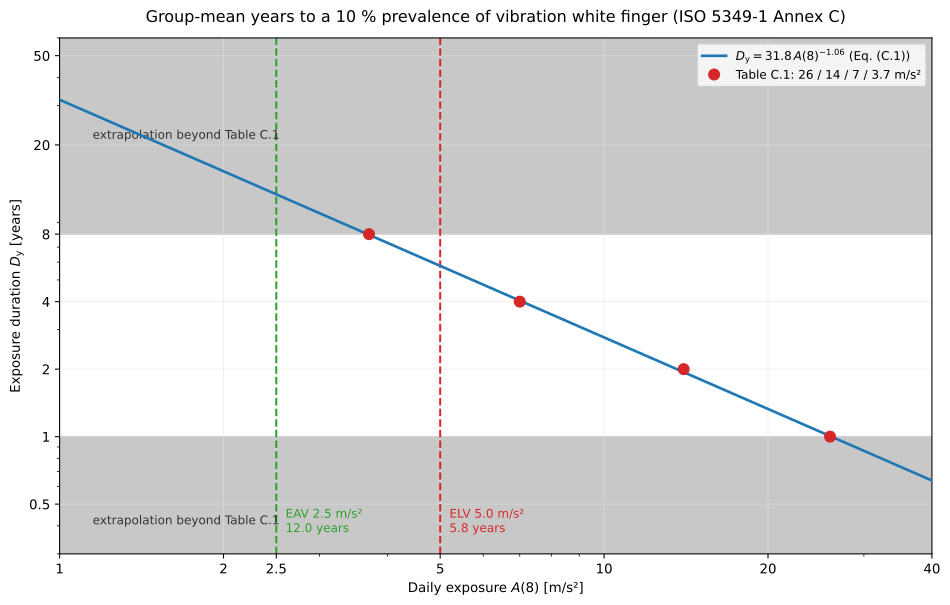

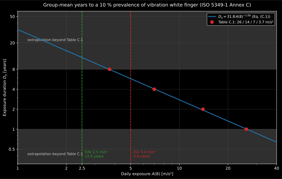
Because the exponent is −1.06, the relation is close to inverse-proportional: halving the daily exposure roughly doubles the group-mean years to a 10 % prevalence. That is the most useful thing it says, and it is why a control measure that takes a tool from 5 to 2.5 m/s² buys about six years.

What bounds this curve. ISO 5349-1 offers Eq. (C.1) as an interpolation rule between the four tabulated points of Table C.1, so the shaded regions of the figure are extrapolation. Four further limits come with it, all of them from the Annex C notes:

• The vascular guidance rests on epidemiological studies of tools whose vibration is predominantly above 30 Hz to 50 Hz — chain saws, grinders, rock drills. Measurements dominated by weighted acceleration at lower frequencies, particularly below about 20 Hz, should be treated with caution (NOTE 2).
• It is a group-mean statement. It does not predict the risk of finger blanching for any particular individual within a group (NOTE 3).
• The underlying groups were exposed to magnitudes up to 30 m/s² for up to 25 years, in near-daily work with one type of tool or process, and the acceleration values come from studies reporting the dominant single-axis component (NOTE 4).
• Deviations occur where the ratio of the vibration total value to the greatest single-axis component departs from typical, and where work-related or environmental factors differ from those of similar occupations (NOTE 5).

Above the curve, “a greater prevalence of finger blanching may be expected” is as far as the standard will go: the 2001 edition deliberately restricted the guidance to the 10 % line to limit the potential for inappropriate use of the relationship. The standards define no safe limit; $A(8)$ and the directive’s action and limit values are the basis for any exposure criterion.

The whole-body counterpart. energy_equivalent_acceleration gives the ISO 2631-1 Eq. (B.3) energy-equivalent magnitude across periods of different magnitude and duration,

$$a_{w,e}=\sqrt{\frac{{\sum }_i{a}_{wi}^2{T}_i}{{\sum }_i{T}_i}},$$

which answers a different question from $A(8)$ on the same inputs: it is a duration-weighted energy average, with no normalisation to an eight-hour day, so it says what a single magnitude would have to be to do the same damage over the same total time, not over a standard day.

# Two hours on rough ground at 0.62 m/s^2, four hours on a haul road at 0.31.
print(round(vibration.energy_equivalent_acceleration([0.62, 0.31], [2 * 3600.0, 4 * 3600.0]), 3))
# 0.438  m/s^2 over the six hours worked ...
print(round(vibration.daily_vibration_exposure([0.62, 0.31], [2 * 3600.0, 4 * 3600.0], kind="wbv").a8, 3))
# ... against A(8) = 0.38 m/s^2, the same energy spread over eight hours

5. The exposure assessment report

A daily exposure is rarely the end of the job: it exists to be written down and compared with the law. DailyVibrationExposure.report() writes a one-page PDF assessment sheet laid out like the hand-arm and whole-body exposure calculators of occupational-hygiene practice (the HSE calculators, the EU Good Practice Guides): the standard-basis line naming the applied ISO method (ISO 5349-1/-2 for hand-transmitted vibration, ISO 2631-1 for whole-body vibration) and the directive it is assessed against, a header grid (company, operator/worker, workplace, instrumentation and calibration), the per-operation exposure analysis (each operation’s vibration magnitude, the hand-arm vector total $a_{hv}$ or the whole-body Directive Part B dominant-axis value $a_{w,max}$, its daily exposure time $T_i$ and the partial exposure $A_i(8)$, closed by the daily total and the combined $A(8)$) with the contribution chart, and the boxed $A(8)$ with its exposure zone.

Because the number exists to be compared with the law, the fiche then assesses $A(8)$ against Directive 2002/44/EC (Article 3): the exposure action value (EAV) and exposure limit value (ELV) for the vibration kind (hand-arm $2.5$ / $5$ m/s²; whole-body $0.5$ / $1.15$ m/s²), each marked exceeded / not exceeded on the value exactly as displayed, with a PASS/FAIL verdict against the limit value. A printed note records that the ISO standards define no safe exposure limit and that reaching the EAV triggers the employer’s control measures and the workers’ entitlement to health surveillance. verbose=True adds each operation’s share of the daily vibration energy, and language="es" renders the Spanish fiche (comma decimals).

The metadata argument accepts a ReportMetadata whose relevant fields for a vibration exposure report are client (the company), specimen (the operator or worker whose exposure was determined), test_room (the workplace), test_date, instrumentation, calibration, and the footer identity laboratory, operator, report_id and notes.

Two of those fields are what ISO 5349-2 clause 9 f) asks for, and they are not free text: instrumentation carries the instrument detail — make, model, serial number and its conformity to ISO 8041-1 — together with the transducer locations and orientations and the mass of the transducer and mount; calibration carries the calibration traceability, the date of the most recent verification test and the result of the before-and-after functionality check of clause 6.3.1. A fiche whose calibration field is empty is not a reportable assessment.

from phonometry import vibration, ReportMetadata

# The ISO 5349-2 Annex E.3 forestry worker: brush-saw (2 h, 4.6 m/s²),
# chain-saw felling (1 h, 6.0 m/s²) and branch stripping (2 h, 3.6 m/s²).
res = vibration.daily_vibration_exposure(
    [4.6, 6.0, 3.6],
    [2 * 3600, 1 * 3600, 2 * 3600],
    kind="hav",
    labels=["Brush-saw clearance", "Chain-saw felling", "Chain-saw branch stripping"],
)

res.report(
    "a8.pdf",
    metadata=ReportMetadata(
        client="Example forestry contractor",
        specimen="Forestry worker (right hand)",
        test_room="Managed woodland, plot 12",
        instrumentation="Hand-arm vibration meter (ISO 8041-1), s/n 0042",
        report_id="EXAMPLE-5349",
    ),
)   # A(8) = 3.61 m/s² -> action zone (EAV exceeded, ELV not), verdict PASS

The example fiche is regenerated with make reports and kept rendered in the repository; click the preview to open the PDF.

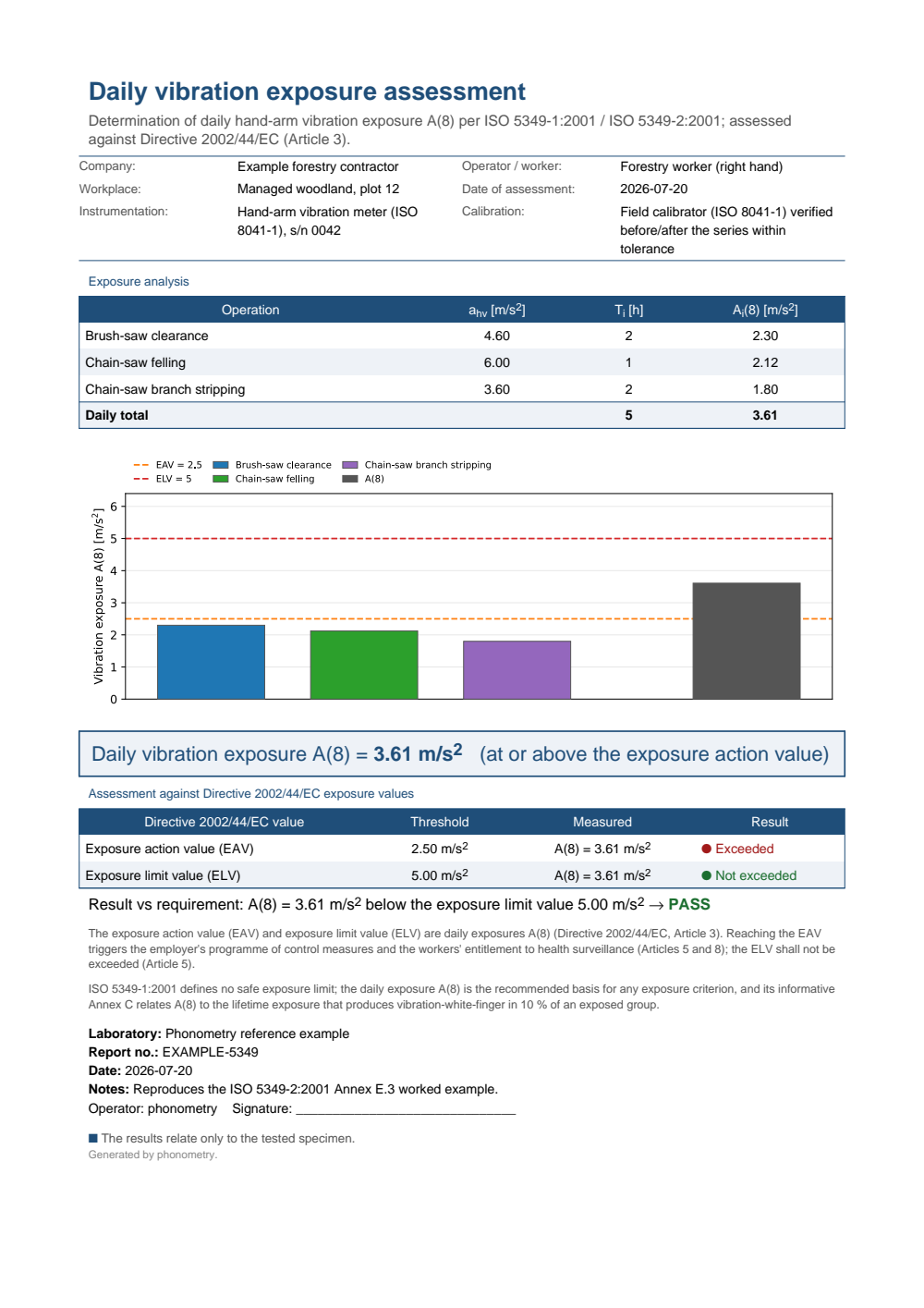
One-page daily vibration exposure assessment fiche: a header with the forestry contractor, the worker, the woodland workplace and the instrumentation, the per-operation exposure-analysis table (brush-saw clearance, chain-saw felling and branch stripping with the vibration total values, daily exposure times and partial exposures A_i(8) closed by the daily-total row), the per-operation contribution chart, the boxed daily exposure A(8) = 3.61 m/s2 in the action zone, and the Directive 2002/44/EC assessment table where the 2.5 m/s2 exposure action value is exceeded and the 5 m/s2 exposure limit value is not, ending in a PASS verdict.

Download the report (PDF)

Daily vibration exposure fiche (DailyVibrationExposure.report), the ISO 5349-2 Annex E.3 hand-arm day with the exposure analysis and the Directive 2002/44/EC assessment.

What this guide covers

• Covered

  ISO 8041-1:2017 as far as it defines the frequency weightings: the Table 3 cascade of analog stages (Formulae (1)-(5)) that frequency_weighting and apply_weighting realise for all nine weightings, reproducing the Annex B design-goal tables. ISO 2631-1:1997 for whole-body vibration, covering the weighted r.m.s. $a_w$ and vibration total value $a_v$ (weighted_acceleration, vibration_total_value), the MTVV, VDV, MSDV and crest-factor dose measures, the clause 6.3.3 comparison ratios, the Annex C comfort scale and the Annex D motion-sickness reading (running_rms, motion_sickness_dose_value), and the Annex B energy-equivalent magnitude (energy_equivalent_acceleration). ISO 2631-2:2003 (Wm), ISO 2631-4:2001 (Wb) and ISO 5349-1/-2:2001 for hand-transmitted vibration, whose vector total, daily exposure $A(8)$ (daily_vibration_exposure, wbv_exposure_basis) and Annex C vibration-white-finger dose relation (hav_vwf_lifetime_years) are implemented too. The Directive 2002/44/EC action and limit values close the assessment, written up by DailyVibrationExposure.report().

• Not covered

  ISO 8041-1’s own subject, the design and type-testing of general purpose vibration meters, is not implemented: only the frequency-weighting definitions are taken from it. ISO 2631-5:2018, the multiple-shock spinal-response and injury-risk model for whole-body vibration, is a separate standard with its own module: see Multiple Shock Vibration for records containing repeated shocks, which the r.m.s. and VDV measures on this page do not substitute for.

See also

• Multiple Shock Vibration: where a record goes once its crest factor and its clause 6.3.3 ratios say the r.m.s. cannot describe it — the ISO 2631-5 spinal-response model, and the seat-pad acquisition this page’s whole-body half points at.
• Sound power from surface vibration: the other thing a surface acceleration is used for, when the question is what the machine radiates rather than what the operator receives.
• Calibration: the before-and-after check of clause 6.3.1 and the traceability the fiche’s calibration field records.
• API reference: vibration.human.exposure.
• Theory: Human vibration: the frequency weightings of ISO 2631-1 and ISO 5349-1, and the running r.m.s., VDV and MTVV definitions.

References

• European Parliament and Council. (2002). Directive 2002/44/EC on the minimum health and safety requirements regarding the exposure of workers to the risks arising from physical agents (vibration) (Directive 2002/44/EC). Official Journal of the European Union. The exposure action and limit values the daily exposure A(8) is assessed against.
• Griffin, M. J. (1996). Handbook of human vibration. Academic Press. ISBN 978-0-12-303041-2. The standard monograph on whole-body and hand-transmitted vibration: the biodynamics, discomfort and health-effect evidence behind the weightings, dose measures and exposure-response guidance on this page.
• International Organization for Standardization. (1997). Mechanical vibration and shock — Evaluation of human exposure to whole-body vibration — Part 1: General requirements (ISO 2631-1:1997). The whole-body evaluation: the weighted r.m.s. and dose measures and the vibration total value.
• International Organization for Standardization. (2001). Mechanical vibration — Measurement and evaluation of human exposure to hand-transmitted vibration — Part 1: General requirements (ISO 5349-1:2001). Hand-transmitted vibration: the general requirements of the evaluation.
• International Organization for Standardization. (2001). Mechanical vibration — Measurement and evaluation of human exposure to hand-transmitted vibration — Part 2: Practical guidance for measurement at the workplace (ISO 5349-2:2001). Hand-transmitted vibration: practical guidance for measurement at the workplace.
• International Organization for Standardization. (2001). Mechanical vibration and shock — Evaluation of human exposure to whole-body vibration — Part 4: Guidelines for the evaluation of the effects of vibration and rotational motion on passenger and crew comfort in fixed-guideway transport systems (ISO 2631-4:2001). Rail ride comfort: the Wb weighting.
• International Organization for Standardization. (2003). Mechanical vibration and shock — Evaluation of human exposure to whole-body vibration — Part 2: Vibration in buildings (1 Hz to 80 Hz) (ISO 2631-2:2003). Vibration in buildings: the Wm weighting applied irrespective of direction (4.4), the highest-axis evaluation (4.5.1), the source categories (4.5.2) and the deliberate absence of acceptable magnitudes.
• International Organization for Standardization. (2016). Mechanical vibration — Laboratory method for evaluating vehicle seat vibration — Part 1: Basic requirements (ISO 10326-1:2016). The semi-rigid accelerometer mounting disc ISO 2631-1 clause 5.3.2 points at for measurements on a seat cushion: its diameter, height, hardness and the metal disc that carries the transducers (5.2.3).
• International Organization for Standardization. (2017). Human response to vibration — Measuring instrumentation — Part 1: General purpose vibration meters (ISO 8041-1:2017). The frequency-weighting definitions and tolerances the implemented weightings follow.
• Mansfield, N. J. (2004). Human response to vibration. CRC Press. ISBN 978-0-415-28239-0. A compact modern textbook on the ISO 2631-1 and ISO 5349 evaluation chains, from perception and comfort to the occupational exposure limits.