Structure-borne sound power of equipment (EN 15657)

Building service equipment (pumps, fans, boilers, sanitary appliances) injects structure-borne sound power into the building structure it is fixed to, which then re-radiates as airborne noise in adjoining rooms. EN 15657:2018 measures it with the reception-plate method: the source is mounted on a plate of known mass per unit area $m$ and area $S$ whose structural loss factor $\eta$ is known, and the plate’s spatial-average vibratory velocity is measured. Formula (14) gives the power injected into that particular plate; the plate-independent source quantities (the equivalent blocked force, Formula 15; the characteristic reception-plate power level $L_{Wsn}$, Formula 17; and the equivalent free velocity and source mobility, Formulae 18/19) are derived from it and are what the EN 12354-5 installed-equipment prediction consumes.

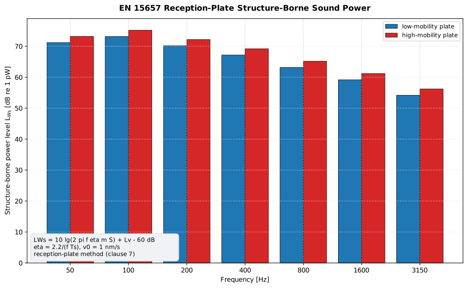
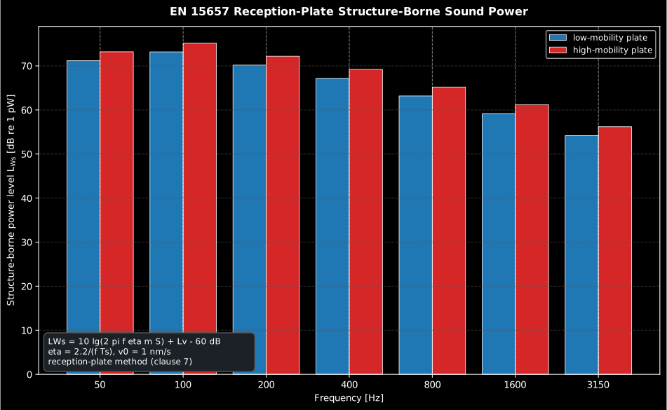
One source, two conforming plates, two answers 12.0 dB apart in every band (67.5 dB against 79.5 dB summed over the bands). The light plate vibrates 35.1 dB harder, but it also dissipates through an $\eta mS$ some 204 times smaller, and $L_{W\mathrm{s}}$ is the power that plate absorbs, not a property of the machine. Read on its own, neither curve describes the source; section 4 is what turns either of them into the plate-independent quantities EN 12354-5 consumes.

Show the code for this figure

import matplotlib.pyplot as plt
import numpy as np
from phonometry import building

# The same pump-like source measured on a conforming low-mobility plate
# (100 mm concrete, 2 300 kg/m3 -> m = 230 kg/m2, 3,15 m x 2,23 m = 7,0 m2,
# Ts = 0,25 s so eta >= 0,08 through 50-100 Hz) and on a conforming
# high-mobility plate (1 mm perforated steel, m = 7,9 kg/m2, 2,0 m2).
bands = np.array([50.0, 100.0, 200.0, 400.0, 800.0, 1600.0, 3150.0])
lv_low = np.array([72.0, 74.0, 71.0, 68.0, 64.0, 60.0, 55.0])

# The light plate's point mobility is 1.1e-2 m/(N.s) against the heavy plate's
# 4.9e-6, so for a source of |Y_S| ~ 1e-3 m/(N.s) its spatial-mean velocity
# level runs 35.1 dB higher: 12.0 dB of that is extra injected power and the
# rest is the plate's much smaller eta*m*S dissipating it.
low = building.reception_plate_power(lv_low, bands, mass_per_area=230.0,
                                     area=7.0, reverberation_time=0.25)
high = building.reception_plate_power(lv_low + 35.1, bands, mass_per_area=7.9,
                                      area=2.0, reverberation_time=0.5)

# One line — the L_Ws(f) bars of one determination with its band-summed total:
low.plot()
plt.show()

# By hand, comparing the two plates from the results' fields:
x = np.arange(bands.size)
fig, ax = plt.subplots()
ax.bar(x - 0.2, low.power_level, width=0.4, label="low-mobility plate")
ax.bar(x + 0.2, high.power_level, width=0.4, label="high-mobility plate")
ax.set_xticks(x, [f"{b:g}" for b in bands])
ax.set(xlabel="Frequency [Hz]",
       ylabel=r"Structure-borne power level $L_{W\mathrm{s}}$ [dB re 1 pW]")
ax.legend()
plt.show()

1. The reception-plate relations

Why a plate at all? Characterising the source by its contact forces directly would mean instrumenting every fixing point in up to six components each (three forces, three moments), on a machine that must keep running normally. The reception plate sidesteps the whole contact problem: let the source run on a resonant plate whose dissipation is known, wait for the steady state, and then the power the plate dissipates equals the power the source injects, over all contacts and components at once. One spatial average of the plate velocity replaces the entire force-measurement problem.

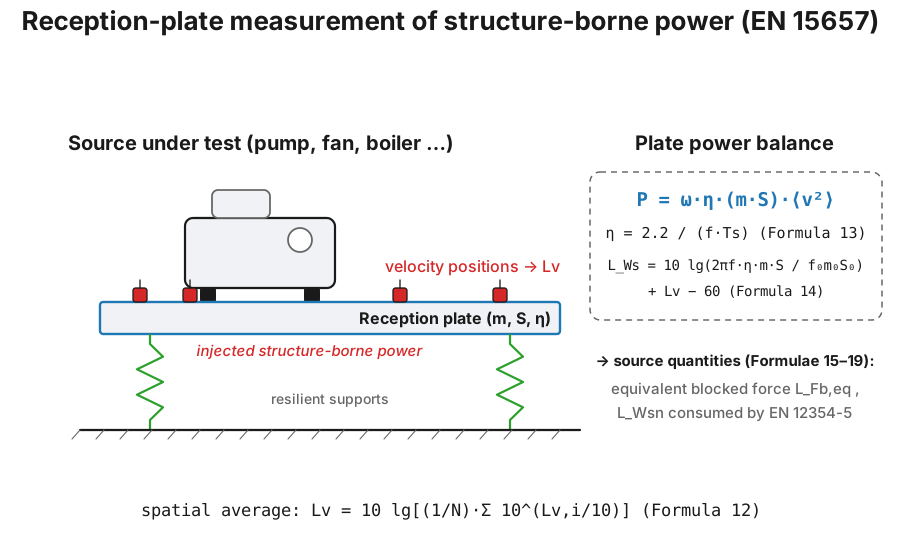
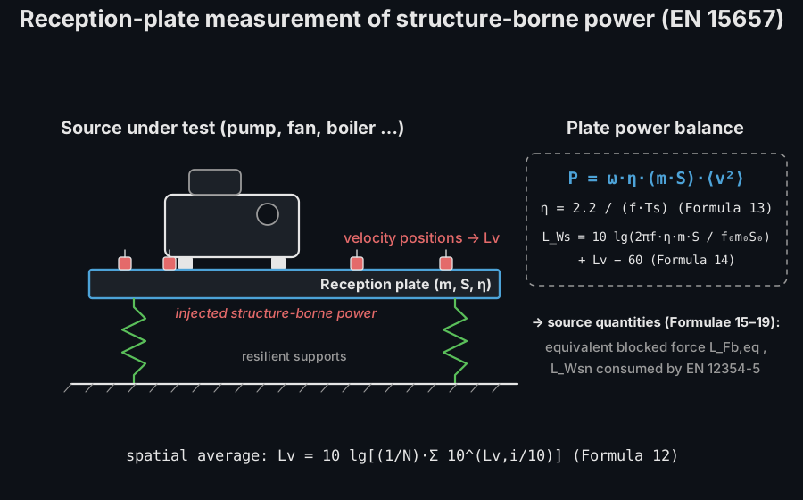
The power a resonant plate dissipates is $P=\omega \eta (mS)⟨v^2⟩$, so the injected power level in one-third-octave bands is (Formula 14)

$$L_{W\mathrm{s}}=10{\log }_{10}\left(\frac{2\pi f\eta mS}{f_0{m}_0{S}_0}\right)+L_v-60[\mathrm{dB}\mathrm{re}1\mathrm{pW}],$$

with references $f_0=1\text{Hz}$, $m_0=1\text{kg}$ (printed as 1 kg; the quantity it normalises is a mass per unit area, so the reference is $1{\text{kg/m}}^2$ — see the errata registry), $S_0=1{\text{m}}^2$; the $-60\text{dB}$ term is $10{\log }_{10}(v_0^2/P_0)$ for the EN 15657 velocity reference $v_0=10^{-9}\text{m/s}$ and $P_0=1\text{pW}$. The plate velocity is the energetic spatial average over the $N$ positions (Formula 12) and the loss factor comes from the structural reverberation time $T_s$ (Formula 13, identical to the ISO 10848 total loss factor):

$$L_v=10{\log }_{10}(\frac{1}{N}\sum 10^{L_{v,i}/10}),\eta =\frac{2.2}{f{T}_s}.$$

import numpy as np
from phonometry import building

bands = np.array([100.0, 200.0, 400.0, 800.0])
lv_i = np.array([88.0, 90.0, 87.0, 89.0, 86.0, 90.0])   # six plate positions @ 200 Hz
print(round(building.spatial_mean_velocity_level(lv_i), 2))    # 88.6 dB re 1 nm/s

# Power level injected into the low-mobility reception plate of clause 7.2.2
# (100 mm concrete, 230 kg/m2 over 7,0 m2, Ts = 0,25 s):
res = building.reception_plate_power(
    velocity_level=np.array([90.0, 87.0, 82.0, 77.0]),
    frequency=bands, mass_per_area=230.0, area=7.0, reverberation_time=0.25,
)
print(np.round(res.power_level, 1))     # [79.5 76.5 71.5 66.5]  per-band L_Ws
print(round(res.total_level, 1))        # 81.8  band-summed level [dB re 1 pW]

res.plot()   # the L_Ws(f) bars with the band-summed total, as in the figure above (needs matplotlib)

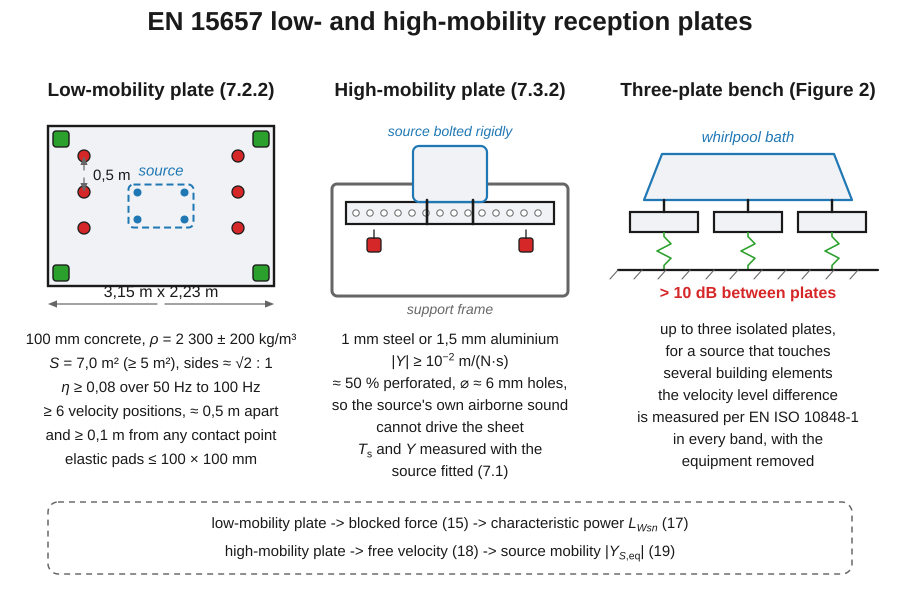
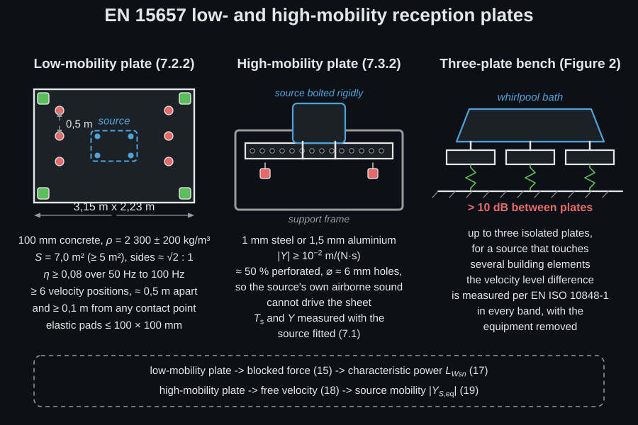
2. Low- and high-mobility plates

Two reception plates bracket the installation conditions, and the standard specifies both.

The low-mobility plate (clause 7.2.2) is concrete of density $(2300\pm 200)$ kg/m³ and thickness $(10\pm 1)$ cm — so about 230 kg/m² — with a minimum area of 5 m² and preferably more than 7 m², a length-to-width ratio near $\sqrt{2}$, and a loss factor of at least 0,08 in the low bands (50 Hz to 100 Hz). Its minimum dimension shall be at least the largest contact spacing of the sample. Every one of those numbers earns its place: the 10 cm concrete plate is the same plate whose characteristic mobility $Y_{R,\infty ,\text{low}}=5\times 10^{-6}$ m/(N·s) anchors Formula (17), so a thinner or lighter plate would break the conversion; the $\sqrt{2}$ aspect ratio spreads the modes so that no band is dominated by a degenerate pair; the loss-factor floor keeps the plate reverberant but well damped, which is what makes $\eta =2,2/(f{T}_s)$ and the steady-state power balance hold — at $T_s=0,25$ s the plate gives $\eta =0,176$ at 50 Hz and 0,088 at 100 Hz, just inside the requirement; and the minimum dimension keeps a multi-contact source from bridging the plate’s edges. A bench may carry up to three mutually isolated low-mobility plates so that a source touching several building elements — a whirlpool bath — can be tested as installed, provided the velocity level difference between the plates, measured per EN ISO 10848-1 with the equipment removed, is more than 10 dB in every band.

The high-mobility plate (clause 7.3.2) is a thin metal sheet designed for a mean point mobility of at least $10^{-2}$ m/(N·s), about 50 % perforated with roughly 6 mm holes; 1 mm steel or 1,5 mm aluminium achieves it, and the sheet is held in a support frame for stability. The perforation is not a weight-saving measure: it exists to stop the sheet being driven by the source’s own airborne sound in a noisy environment, which would be indistinguishable from structure-borne injection. The sample is fixed rigidly to this plate.

Mounting (clause 7.2.3). On the low-mobility plate the source goes towards the plate centre, away from the vibration nodes, so that the point mobility, the free velocity and the blocked force vary as little as possible over its contacts — the reception-plate method works best on sources whose contacts are alike. The source is mounted exactly as its manufacturer prescribes for real buildings, and the mounting is described in full in the test report.

Which plate gives which quantity. The equivalent blocked force (Formula 15) and the characteristic reception-plate power level (Formula 17) are read from the low-mobility plate. The equivalent free velocity (Formula 18) and, with the blocked force, the source mobility (Formula 19) need the high-mobility plate — whose reverberation time and point mobilities must therefore be measured with the source attached. The pair brackets the installation: a real building element sits between the two, and the gap between the two determinations is what says whether the machine behaves as a force source or as a velocity source. The plate-injected power plus the plate’s point mobility (see mechanical mobility) yield the source description for the EN 12354-5 model through the conversion chain below.

Caution

Two velocity references share the symbol $v_0$. EN 15657 and EN 12354-5 refer velocity levels to $v_0=10^{-9}$ m/s (1 nm/s); ISO 9611 and ISO/TS 7849 refer them to $5\times 10^{-8}$ m/s (50 nm/s). The two differ by $20{\log }_{10}(50)=33.98$ dB, so a free velocity level taken from an ISO 9611 report must be reduced by 34.0 dB before it enters Formula (18) or any EN 12354-5 quantity. Section 4 below uses both references, a few lines apart.

3. Running the measurement

Everything that decides whether a reception-plate determination is valid sits in clause 7.1, and none of it is in the formulae.

Transducers and positions. Accelerometers calibrated to ISO 16063-21 and mounted to ISO 5348. The spatial mean velocity level and the structural reverberation time are measured as EN ISO 10848-1 prescribes. There shall be not fewer than six measurement positions, about 0,5 m apart and at least 0,1 m from the equipment’s contact points — the clearance is what makes the mean a plate average instead of a near-field reading of the contact, and the spacing is what makes six positions sample different modal patterns rather than one. The number and the location of the positions are validated with the Annex C power-substitution method described at the end of this section.

Background vibration. Velocity levels are expressed in dB re $10^{-9}$ m/s and corrected for background vibration by the same procedure used for sound pressure levels, in accordance with EN ISO 10140-3: measure the plate with the source off, and correct or reject the band according to the margin. A plate standing on a laboratory floor picks up traffic and plant long before a microphone does, and the correction is the only thing between that and a source spectrum that is really the building’s.

The loss factor. $T_s$ is a structural decay measured on the plate itself, feeding $\eta =2,2/(f{T}_s)$. Formula (14) is linear in $10\lg \eta$, so an error in $T_s$ moves $L_{W\mathrm{s}}$ decibel for decibel — it is the single most sensitive input on the page. The loading rule follows the plate: on the low-mobility plate there should be no significant difference whether $T_s$ and the point mobilities are measured with or without the equipment attached; the high-mobility plate is dynamically loaded by the equipment, so both $T_s$ and the point mobilities shall be measured with the source fitted.

Mobilities. The plate’s point mobilities are measured at the source’s contact points per ISO 7626-1, restricted to single-point translational excitation normal to the plate per ISO 7626-2 (impact excitation per ISO 7626-5 is allowed), in narrow bands and then reduced to one-third octaves. The receiver is not dynamically loaded while this is done; a source, by contrast, is isolated per ISO 9611 or freely suspended.

Operating conditions are part of the result, not of the setup. Formula (14) equates injected with dissipated power only in the steady state, so an intermittent or cyclic machine has to be run in a defined condition and the condition reported: clause 10 requires the free velocity, the blocked force, the source mobility and the characteristic power to be stated per tested operating condition and per source component. The standard’s own whirlpool-bath schedule in Annex B is the model to copy.

What the numbers are worth. The 2010 interlaboratory test (clause 8.1) gives a standard deviation of about 3 dB per one-third-octave band for repeatability within a laboratory and about 4 dB for reproducibility between laboratories, for the isolated low-mobility plate with a reference source of controlled internal forces. That is the scale against which a 1 dB difference between two determinations means nothing.

Three failure modes are silent, and each is why one of the requirements above exists. The source’s own airborne sound can drive the plate — which is why the high-mobility plate is about half perforated. A loss factor measured on the bare plate can be carried into the high-mobility case, where the standard requires the source to be attached, and the error goes straight into $L_{W\mathrm{s}}$. And a machine that has not reached steady state, or that is measured over a cycle average without saying so, produces a number that no other laboratory can reproduce.

When the plate cannot be isolated: power substitution

Annex C is normative and covers three situations: validating the measurement positions on either plate; determining the injected power in the laboratory on a non-isolated low-mobility plate, when connecting the sample to an isolated one is difficult or impossible (waste-water pipes fixed to both a wall and a floor); and determining it in situ, for equipment such as lifts that can only be tested where it is installed.

The plate is first excited by a calibrated structural source of known power $P_{\text{cal}}$ — an electrodynamic shaker with broadband noise or an impact hammer, as EN ISO 10848-1 describes — and its mean-square velocity measured; replacing the calibrated source by the sample and measuring again gives $P_{\text{source}}=⟨v_{\text{source}}^2⟩P_{\text{cal}}/⟨v_{\text{cal}}^2⟩$ (Formula C.1). The known power is injected at three points on a low-mobility plate — one central, one 0,5 m from an edge and one 0,5 m from a corner — or at at least two points away from the contacts on a high-mobility plate, each averaged over the same six or more receiver positions and combined energetically (Formula C.2). The standard notes that the substitution is probably valid only up to about 1 kHz.

This is how lifts and stack pipes get a characteristic power at all, and it is also the reason a coupled wall or floor cannot simply be treated as a reception plate: energy returning from the structure the plate is attached to makes the plate power balance wrong, and only the substitution measures round it.

4. From plate power to source quantities (Formulae 15–19)

The plate-injected $L_{W\mathrm{s}}$ is not a source descriptor: the same source injects a different power into a different receiver. EN 15657 derives the plate-independent quantities: the equivalent blocked force level (Formula 15, re $F_0=10^{-6}\text{N}$, not the 1 N reference of the ISO 16283-2 impact force exposure level, 120 dB away) from the low-mobility plate,

$$L_{Fb,eq}=L_{Ws,\mathrm{low}}-10{\log }_{10}\frac{\mathrm{Re}\{Y_{R,\mathrm{low},\mathrm{eq}}\}}{Y_0},$$

the characteristic reception-plate power level that EN 12354-5 consumes (Formula 17), referred to the standard 10 cm concrete plate of characteristic mobility $Y_{R,\infty ,\text{low}}=5\times 10^{-6}\text{m/(N⋅s)}$ (clause 7.2.4),

$$L_{Wsn}=L_{Fb,eq}+10{\log }_{10}\frac{Y_{R,\infty ,\mathrm{low}}}{Y_0},$$

and, from the high-mobility plate, the equivalent free velocity level (Formula 18, re $10^{-9}\text{m/s}$) and the source mobility $|Y_{S,\text{eq}}|$ (Formula 19). The EN 12354-5 Annex I mobility correction (installed_power_from_reception_plate, see installed structure-borne sound) then refers $L_{Wsn}$ to the actual receiving element.

from phonometry import building

# EN 12354-5 Annex I.3 (flushing cistern, wall contact, 63 Hz): measured on a
# plate of Y = 5.34e-6 m/(N·s); the wall's characteristic mobility is 24.1e-6.
lfb = building.equivalent_blocked_force_level(61.7, 5.34e-6)      # Formula (15)
lwsn = building.characteristic_reception_plate_power(lfb)         # Formula (17)
inst = building.installed_power_from_reception_plate(lwsn, 24.1e-6)  # Annex I
print(round(float(lwsn), 1), round(float(inst), 1))         # 61.4 68.2  (Table I.8)

# The same Annex I correction taken to the SOURCE mobility instead gives the
# plate-independent characteristic power level EN 12354-5 asks for as input:
lwsc = building.installed_power_from_reception_plate(lwsn, 1.0e-3)
print(round(float(lwsc), 1))                                # 84.4  L_Ws,c

# Free velocity (Formula 18) + blocked force close the source mobility (19).
# The 1.0e-2 m/(N.s) is EN 15657's minimum specified high-mobility plate
# mobility, not an arbitrary number.
lvf = building.equivalent_free_velocity_level(70.0, 1.0e-2)
print(float(building.source_mobility_from_levels(lvf, lfb)))      # |Y_S,eq| in m/(N·s)

Read the chain in order. The cistern injects 61.7 dB into the measurement plate; stripping that plate’s mobility leaves an equivalent blocked force, and re-expressing the same force on the standard 10 cm concrete plate of $Y_{R,\infty ,\text{low}}=5\times 10^{-6}\text{m/(N⋅s)}$ gives $L_{Wsn}=61.4$ dB — the number a manufacturer may declare. Referring the same force to the actual receiving wall ($Y=24.1\times 10^{-6}$) adds $10{\log }_{10}(24.1/5.0)=6.8$ dB and gives 68.2 dB. That step is the section’s whole lesson: a light, high-mobility receiver accepts more power from the same source, so a declared $L_{Wsn}$ compares machines and is never the power a particular building will see.

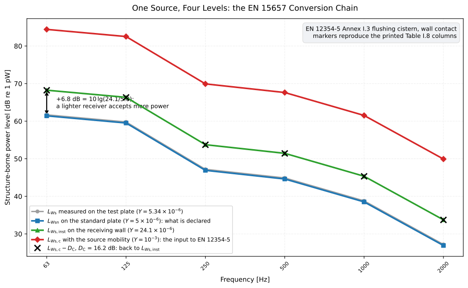
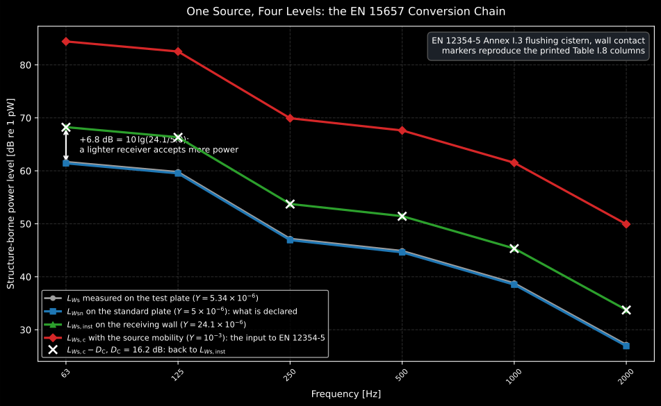
The same source, four different levels, and only one of them describes the machine. Read upward from the grey curve: what the test plate measured, then the declared $L_{Wsn}$ on the standard 10 cm plate, then the two branches of the Annex I correction — the receiving wall’s 68.2 dB and the plate-independent 84.4 dB. The crosses are $L_{Ws,c}-D_C$, and they land on the installed curve, which is the arithmetic the two pages share. The 6.8 dB step at every band is $10\lg (24.1/5.0)$: nothing about the cistern changed, only what it was bolted to.

Show the code for this figure

import matplotlib.pyplot as plt
import numpy as np
# `building` as imported by the snippet above.

bands = np.array([63.0, 125.0, 250.0, 500.0, 1000.0, 2000.0])
l_ws = np.array([61.7, 59.8, 47.2, 44.9, 38.8, 27.2])     # on the test plate
l_fb = building.equivalent_blocked_force_level(l_ws, 5.34e-6)
l_wsn = building.characteristic_reception_plate_power(l_fb)
installed = building.installed_power_from_reception_plate(l_wsn, 24.1e-6)
characteristic = building.installed_power_from_reception_plate(l_wsn, 1.0e-3)

fig, ax = plt.subplots()
ax.semilogx(bands, l_ws, "-o", label="measured on the test plate")
ax.semilogx(bands, l_wsn, "-s", label=r"$L_{W\mathrm{sn}}$, the declared value")
ax.semilogx(bands, installed, "-^", label=r"$L_{W\mathrm{s,inst}}$ on the wall")
ax.semilogx(bands, characteristic, "-D",
            label=r"$L_{W\mathrm{s,c}}$, the EN 12354-5 input")
ax.semilogx(bands, characteristic - 16.2, "x",
            label=r"$L_{W\mathrm{s,c}} - D_\mathrm{C}$")
ax.set(xlabel="Frequency [Hz]",
       ylabel="Structure-borne power level [dB re 1 pW]")
ax.legend()
plt.show()

Caution

Two quantities come out of the same correction; do not confuse them. With the receiver mobility it gives the installed power level $L_{Ws,\mathrm{inst}}=68.2$ dB. With the source mobility it gives the plate-independent characteristic power level $L_{Ws,c}=84.4$ dB, and that is what EN 12354-5 takes as its input, from which it subtracts the coupling term $D_C=16.2$ dB to arrive back at the same 68.2 dB. Feed EN 12354-5 the 84.4, never the 68.2: carrying 68.2 forward as the characteristic power level subtracts $D_C$ a second time and lands 16 dB low, with no error raised.

The direct source-side counterpart is the ISO 9611 free velocity level (re $v_0=5\times 10^{-8}\text{m/s}$, the 50 nm/s reference of the callout above, not the 1 nm/s of Formula 14) measured at the contact points of resiliently mounted machinery; its equation (9) position average is mean_free_velocity_level().

5. The characterization report (.report())

A characterization ends as a document. The StructureBornePowerResult exposes a .report() method that writes a one-page PDF fiche laid out like a sound-power test sheet: the standard-basis line naming the EN 15657:2018 reception-plate method (Formula 14), an optional metadata header (client, source equipment, test environment, instrumentation, climate, date), a per-band table (nominal octave/one-third-octave frequency, the spatial mean plate velocity level $L_v$ and the injected structure-borne sound power level $L_{W\mathrm{s}}$), the $L_{W\mathrm{s}}(f)$ spectrum with a nominal band axis, and a boxed band-summed total $L_{W\mathrm{s}}$ (dB re 1 pW) with the plate mass per area $m$ and area $S$.

The metadata is supplied through a ReportMetadata, whose applicable fields here are the source equipment (specimen), the test environment (test_room), the client, the instrumentation, the temperature, relative humidity and ambient pressure, the date of test (test_date) and the footer identity (laboratory, operator, report_id, notes); the plate mass and area come from the result itself. Supplying requirement adds a PASS/FAIL verdict against a declared upper limit on the total $L_{W\mathrm{s}}$ (a power emission is a quantity where less is better, so the source passes at or below the limit). verbose=True adds the plate loss factor $\eta$ column to the table. language="es" renders the Spanish fiche with comma decimals. The basis strip states Formula 14 and reminds that the plate-injected level must be converted to the plate-independent source quantities (Formulae 15/17) before it feeds EN 12354-5.

import numpy as np
from phonometry import ReportMetadata, reception_plate_power

freqs = np.array([125, 250, 500, 1000, 2000, 4000], float)
lv = np.array([70.0, 72, 68, 64, 60, 55])   # spatial mean plate velocity level [dB]
res = reception_plate_power(               # the clause 7.2.2 low-mobility plate
    lv, freqs, mass_per_area=230.0, area=7.0, reverberation_time=0.25,
)

res.report(
    "structure_borne_power.pdf",
    metadata=ReportMetadata(
        client="Example building services contractor",
        specimen="Circulation pump (wall-mounted)",
        test_room="Reception-plate test rig (heavy concrete plate)",
        laboratory="Phonometry reference example",
        report_id="EXAMPLE-15657",
    ),
)   # total L_Ws ~ 65 dB re 1 pW

The example fiche is regenerated with make reports and kept rendered in the repository; click the preview to open the PDF.

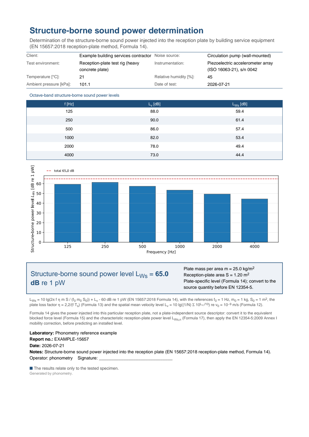
One-page EN 15657:2018 reception-plate structure-borne sound power fiche: a header with the client, the source equipment, the reception-plate test rig and the accelerometer and climate, the octave-band table (125 Hz to 4 kHz) of spatial mean plate velocity levels Lv and injected structure-borne sound power levels L_Ws, the L_Ws(f) spectrum with a nominal band axis, and the boxed band-summed total L_Ws (dB re 1 pW) with the plate mass per area m = 230 kg/m2 and area S = 7.00 m2 of the clause 7.2.2 low-mobility plate, closed by a basis strip stating the Formula 14 relation and the conversion to the plate-independent source quantities required before EN 12354-5.

Download the report (PDF)

Structure-borne sound power fiche (StructureBornePowerResult.report), an EN 15657 reception-plate characterization with the boxed total L_Ws.

What this guide covers

• Covered

  EN 15657:2018’s reception-plate method: the spatial mean velocity level (spatial_mean_velocity_level, Formula 12), the plate loss factor (plate_loss_factor, Formula 13) and the plate-injected power level (reception_plate_power, structure_borne_power_level, Formula 14). Also the plate-independent source-quantity chain: the equivalent blocked force level (equivalent_blocked_force_level, Formula 15), the characteristic reception-plate power level (characteristic_reception_plate_power, Formula 17), the equivalent free velocity level (equivalent_free_velocity_level, Formula 18) and the source mobility (source_mobility_from_levels, Formula 19). Also covered is ISO 9611:1996’s position-averaged free velocity level, equation (9) (mean_free_velocity_level).

• Not covered

  Formula 16, the equivalent point mobility of a plate as the arithmetic mean of $\mathrm{Re}(Y)$ over its contact points, is not implemented: the functions above take an already-known plate_mobility as input rather than deriving it from per-point measurements. The Annex C power-substitution method is likewise not implemented — the library takes an already-averaged $L_v$, so a substitution determination must be reduced to a plate power level by hand (Formulae C.1/C.2) before structure_borne_power_level is used. Nor does anything here check the facility: the plate’s dimensions, density, aspect ratio and loss factor, the position count and clearances, the background correction and the operating conditions are the operator’s responsibility, and a value computed from a non-conforming plate is returned without complaint. Of ISO 9611:1996, only the equation (9) position average is implemented; the rest of the standard is cited as the source-side counterpart, not implemented.

See also

• API reference: building.measurement.structure_borne_power.
• Theory: Point mobilities and radiation efficiency: the point mobility, the source-receiver mismatch and the injected power they define.

References

• Cremer, L., Heckl, M., & Petersson, B. A. T. (2005). Structure-borne sound: Structural vibrations and sound radiation at audio frequencies (3rd ed.). Springer. https://doi.org/10.1007/b137728The plate power balance and the source-receiver mobility framework behind the reception-plate method and its Formula 15-19 source quantities. ISBN 978-3-540-22696-3.
• European Committee for Standardization. (2018). Acoustic properties of building elements and of buildings — Laboratory measurement of structure-borne sound from building service equipment for all installation conditions (EN 15657:2018). The reception-plate method (clause 7): the spatial mean velocity level (Formula 12), the plate loss factor η = 2.2/(f·Ts) (Formula 13), the plate-injected power level L_Ws (Formula 14, plate velocity levels referred to v₀ = 10⁻⁹ m/s) and the source-quantity chain: equivalent blocked force (Formula 15), characteristic reception-plate power level (Formula 17, Y_R,∞,low = 5·10⁻⁶ m/(N·s)), equivalent free velocity (Formula 18) and source mobility (Formula 19). Conformance is anchored on the resonant-plate power balance P = ω·η·(m·S)·⟨v²⟩ (of which Formula 14 is the level), the loss-factor identity, and the EN 12354-5 Annex I.3 Table I.8 conversion of the flushing-cistern source. The linked catalogue record is the UNE page for UNE-EN 15657:2018.
• International Organization for Standardization. (1996). Acoustics — Characterization of sources of structure-borne sound with respect to sound radiation from connected structures — Measurement of velocity at the contact points of machinery when resiliently mounted (ISO 9611:1996). The free-velocity source characterization that complements the reception-plate quantities: equation (9), reference velocity v₀ = 5·10⁻⁸ m/s.