Field Insulation Measurement (ISO 16283)
Standards: ISO 16283ISO 717ISO 12999Key references: Hopkins 2007Vigran 2008
This guide continues from the Room Acoustics guide: the same impulse response, measured either side of a partition, yields its sound insulation. This page covers the engineering-grade measurement of ISO 16283 in the finished building: the airborne level differences , and , the impact levels and , the field test report, and the ISO 12999-1 uncertainty that qualifies every field value. Three close relatives have guides of their own: the reference-curve engine behind every single number in Insulation Ratings (ISO 717), the building envelope in Façade Sound Insulation, and the quick octave-band route in Sound Insulation Survey Method (ISO 10052). The laboratory characterisation of an element lives in Laboratory Insulation Measurement and the prediction of in-situ performance in Predicting Sound Insulation (EN 12354).
How do I compute DnT and R’ from a field measurement in Python?
Section titled “How do I compute DnT and R’ from a field measurement in Python?”Energy-average the source- and receiving-room levels per one-third-octave band
across the microphone positions of one loudspeaker position, correct the
receiving room for background noise, and pass them, with the receiving-room
reverberation time, to
building.airborne_insulation(l1, l2, t2, area=S, volume=V). The result
carries the raw level difference d, the standardized dnt and, when area
and volume are given, the apparent r_prime. If a single loudspeaker was
moved between positions, repeat that for each position and combine the
results with Formula (6), not the levels; see
Taking the measurement.
Impact measurements go through
building.impact_insulation(li, t2, volume=V), and either spectrum is rated
with building.weighted_rating / weighted_impact_rating.
Field airborne insulation (ISO 16283-1)
Section titled “Field airborne insulation (ISO 16283-1)”To rate a wall or floor, measure the energy-average level in the source room () and the receiving room () per one-third-octave band and form the level difference . Two normalisations make it comparable between rooms. The standardized level difference references the receiving-room reverberation time to s (so with s, exactly), and the apparent sound reduction index normalises by the partition area and the Sabine absorption area :
Positions are energy-averaged with .
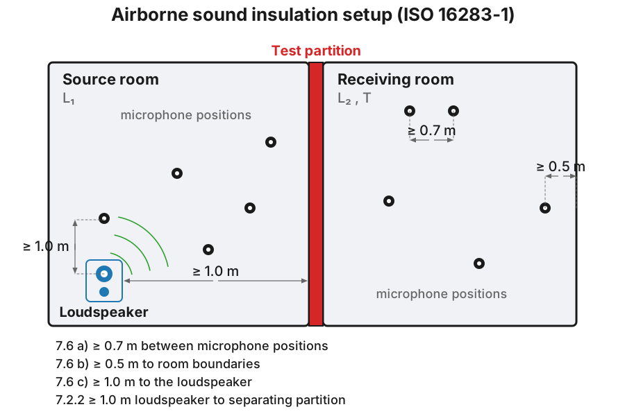
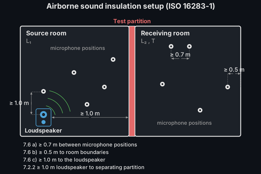
The prime on is a convention, not decoration: primed quantities (, , ) are measured in the building and include every flanking path, while the unprimed and are laboratory properties of the element alone, measured with flanking suppressed. The full lab-to-field map lives in Laboratory Insulation Measurement; the prediction that bridges the two is EN 12354.
One measurement yields all three quantities, so which one goes on the report is a regulatory question, not a measurement one. describes the room pair as the occupants experience it, and that is what most national codes for dwellings state their requirements in. describes the partition, normalised by its area, and is what a comparison against a laboratory or an EN 12354 prediction needs. Measure once, then report the quantity the requirement is written in and say which it is: an cannot be checked against a limit without converting through the room’s and the partition area first; see Spanish Building Code (CTE DB-HR), which states its between-rooms requirement in and its partition-wall requirement in .
import numpy as npfrom phonometry import building
# Energy-average several microphone positions in one room (dB)print(round(float(building.energy_average_level([60.0, 66.0])), 1))   # 64.0
# Field insulation per band; area S and volume V add R'l1 = np.full(16, 80.0)                                # source-room levelsl2 = np.full(16, 40.0)                                # receiving-room levelst2 = np.full(16, 0.5)                                 # receiving-room T (s)ins = building.airborne_insulation(l1, l2, t2, area=10.0, volume=50.0)print(round(float(ins.dnt[0]), 1))                   # 40.0  (= D since T = T0)print(round(float(ins.r_prime[0]), 1))               # 38.0
# The single number comes from the ISO 717-1 engine of the ratings guideprint(building.weighted_rating(ins.dnt).rating)      # 40  DnT,wprint(building.weighted_rating(ins.r_prime).rating)  # 38  R'w
Compute l1, l2 and t2 on the same 16 one-third-octave bands from
100 Hz to 3150 Hz (obtain t2 from
room_parameters(ir, fs, limits=(100, 3150), fraction=3).t30, for example) and
pass them to airborne_insulation. Feed that function’s dnt (or r_prime)
spectrum to weighted_rating, so every band aligns index-by-index with the
ISO 717-1 reference curve.
The scale is worth carrying: for a separating wall or floor between dwellings, national requirements typically sit around dB and rarely below 45 dB, so the 40 dB of this deliberately flat example would fail every one of them. Higher is better for an airborne quantity, and 5 dB is roughly the step between a construction that works and one that generates complaints.
airborne_insulation() parameters
Section titled “airborne_insulation() parameters”| Parameter | Type | Units | Range / default | Notes |
|---|---|---|---|---|
l1 | 1D or 2D array | dB | one/band, or (positions, bands) | Source-room levels (2D is energy-averaged) |
l2 | 1D or 2D array | dB | same band count | Receiving-room levels |
t2 | 1D array | s | > 0, one per band | Receiving-room reverberation time |
area | float, optional | m² | > 0, with volume | Partition area (enables ) |
volume | float, optional | m³ | > 0, with area | Receiving-room volume |
t0 | float | s | default 0.5 | Reference reverberation time |
airborne_insulation() returns an AirborneInsulationResult (d, dnt,
r_prime or None). The reference-curve engine that turns any of those
spectra into , or , its spectrum adaptation terms and its
enlarged-range variants are in
Insulation Ratings (ISO 717).
Taking the measurement (ISO 16283-1 Clauses 7 and 9)
Section titled “Taking the measurement (ISO 16283-1 Clauses 7 and 9)”The functions consume band levels; the standard says where those levels come from, and getting that wrong changes the answer more than any of the arithmetic above.
The source (Clause 7.1, 7.2). Sound is generated with loudspeakers operated simultaneously in at least two positions, or with a single loudspeaker moved to at least two positions. Multiple loudspeakers must be of the same type, driven at the same level by similar but uncorrelated signals, and each must meet the Annex A directivity requirement. The signal is steady with a continuous spectrum, and the energy-average source-room level must not change by more than 8 dB between adjacent one-third-octave bands, at least above 100 Hz: shape the spectrum (a graphic equaliser is usually needed) or fall back to serial band-limited measurements. Loudspeakers stand at least 0.5 m from any boundary, preferably at least 1.0 m from the separating partition, measured to the centre of the nearest speaker unit; different positions must not lie in planes parallel to a boundary less than 0.7 m apart, must be at least 0.7 m apart, and at least two of them at least 1.4 m apart. When the floor is the test element and the loudspeaker is in the upper room, its base sits at least 1.0 m above the floor.
The microphones (Clause 7.3). A minimum of five positions per room, and, with a single loudspeaker moved between positions, five per room per loudspeaker position. No two positions may lie in the same plane relative to the room boundaries, and the set must not form a regular grid.
Correcting for background noise (Clause 9.2)
Section titled “Correcting for background noise (Clause 9.2)”Measure the receiving room again with the source off, at the same positions and with the same averaging, and compare band by band with the combined signal-plus-background level :
- margin dB: use unchanged;
- dB: subtract the background in energy, (Formula 14), with both levels first reduced to one decimal place;
- margin dB: apply the fixed 1.3 dB correction, and flag the band in the report as being at the limit of measurement.
import numpy as np
l2_sb = np.array([44.0, 41.0, 39.5, 38.0])   # receiving room, source onl2_bg = np.array([30.0, 33.0, 31.0, 34.0])   # receiving room, source offmargin = l2_sb - l2_bg                       # 14.0  8.0  8.5  4.0 dB
formula_14 = 10 * np.log10(10 ** (l2_sb / 10) - 10 ** (l2_bg / 10))l2_corr = np.where(margin >= 10.0, l2_sb,                   np.where(margin > 6.0, formula_14, l2_sb - 1.3))print(np.round(l2_corr, 2))     # [44.   40.25 38.84 36.7 ]  <- last band flagged
building.background_correction exists, but it implements the ISO 10140-4
laboratory rule used on
Laboratory Insulation Measurement,
whose upper threshold is 15 dB rather than 10 dB. Applied to field data it
subtracts energy in the 10-15 dB margin band where ISO 16283-1 asks for
nothing (up to 0.458 dB at a 10 dB margin), and since it acts on the
receiving room that lands as over-reported insulation, band for band, in .
Use the three-regime expression above for field levels.
Averaging over loudspeaker positions (Formula 6)
Section titled “Averaging over loudspeaker positions (Formula 6)”With multiple loudspeakers operating simultaneously (Clause 7.3.3) there is one measurement: energy-average the positions in each room, correct for background noise, and form or once. With a single loudspeaker moved between positions (Clause 7.3.4) the standard does not average the levels across loudspeaker positions. It forms the result for each position and averages the results as transmission factors,
which weights the worst position most. The two routes are not the same number:
import numpy as np# `building` is the import of the airborne-insulation block above.
t2 = np.full(16, 0.5)l1a, l2a = np.full(16, 80.0), np.full(16, 40.0)   # loudspeaker position 1l1b, l2b = np.full(16, 83.0), np.full(16, 37.0)   # loudspeaker position 2
# Clause 7.3.4: one result per loudspeaker position, combined by Formula (6).a = building.airborne_insulation(l1a, l2a, t2, area=10.0, volume=50.0)b = building.airborne_insulation(l1b, l2b, t2, area=10.0, volume=50.0)dnt = -10 * np.log10(np.mean(10.0 ** (-np.vstack([a.dnt, b.dnt]) / 10.0), axis=0))print(round(float(dnt[0]), 1), building.weighted_rating(dnt).rating)        # 42.0 42
# Averaging the levels first instead: a different, more flattering number.l1m = building.energy_average_level(np.vstack([l1a, l1b]), axis=0)l2m = building.energy_average_level(np.vstack([l2a, l2b]), axis=0)naive = building.airborne_insulation(l1m, l2m, t2, area=10.0, volume=50.0)print(round(float(naive.dnt[0]), 1), building.weighted_rating(naive.dnt).rating)  # 43.0 43
Small rooms: the low-frequency procedure (Clause 8)
Section titled “Small rooms: the low-frequency procedure (Clause 8)”This one is easy to miss and it is mandatory. When the source and/or receiving room has a volume smaller than 25 m³ (calculated to the nearest cubic metre, so a 25.4 m³ bedroom does not trigger it and a 24.4 m³ one does), the 50 Hz, 63 Hz and 80 Hz one-third-octave bands must additionally be measured in the corners of that room (Clause 6 and Clause 8.1). Most European bedrooms and every bathroom fall under the threshold, so this is the normal case in dwelling work, not an edge case. It is in addition to the default procedure, not instead of it, and the same 25 m³ rule governs the reverberation time.
The reason is stated in the standard’s own NOTE 1: at those frequencies a small room’s field is modal, the spatial variation is large, and the central-zone average is neither repeatable nor representative of what an occupant hears. A modal pressure maximum always sits in a corner, so corner measurements bound the field from above.
How the corners enter the result (Clause 8.5). For each of the three bands independently, take the highest of the measured corners, which may be a different corner in each band, as ; with several loudspeaker positions, energy-average those per-position maxima (Formula (12)). Then combine with the default-procedure average in a 1:2 weighting (Formula (13)):
replaces in those three bands, and or is then formed exactly as before. Under the receiving room’s own trigger, Clause 10.4 also stops the 50 Hz, 63 Hz and 80 Hz one-third-octave reverberation times being measured and puts one 63 Hz octave band value in their place.
# `np` and `building` are the imports of the blocks above.
# 50, 63, 80 Hz. Four corners measured in a 22 m3 receiving room, one# loudspeaker position; the default central-zone average alongside.corners = np.array([                      # rows: corners, columns: the 3 bands    [52.1, 55.4, 49.8],    [54.6, 53.0, 51.2],    [51.0, 56.9, 50.4],    [53.3, 54.1, 52.7],])l_default = np.array([49.5, 51.2, 48.6])
# Clause 8.5: the loudest corner, band by band (Formula (12) at q = 1).l_corner = building.corner_level(corners)print(l_corner)                           # [54.6 56.9 52.7]  (three different corners)
l_lf = building.low_frequency_level(l_default, l_corner)   # Formula (13)print(np.round(l_lf, 1))                  # [51.9 54.  50.4]print(np.round(l_lf - l_default, 1))      # [2.4 2.8 1.8]  dB above the default
print(building.low_frequency_procedure_applies(22.0))   # Trueprint(building.low_frequency_procedure_applies(25.4))   # False, rounds to 25
In a whole measurement the two halves travel together in a
LowFrequencyProcedure, which airborne_insulation() applies to the band
vector for you, and impact_insulation() and facade_insulation() take the
same object under a low_frequency= keyword.
They warn when you forget, everywhere the procedure is allowed: airborne,
impact, and the loudspeaker façade methods. A road-traffic façade stays silent
because Clause 6 of ISO 16283-3 gives it the default procedure and nothing
else, so there is nothing to have forgotten. A volume that rounds below
25 m³ beside a frequencies vector naming any of the three bands tells
the function
that Clause 8.1 (Clause 7.3.1 for the loudspeaker façade) is in force, and
with no procedure to run it says so with a
LowFrequencyWarning rather than returning a number that is not the ISO 16283
one. The corner geometry, the
sampling requirements, the differences between the three parts and a worked
measurement with its rating are all in a guide of their own:
Small Rooms: the ISO 16283 Low-Frequency Procedure.
Field impact insulation (ISO 16283-2)
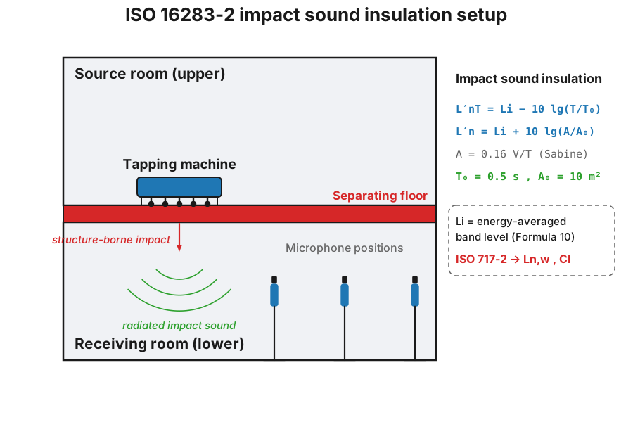
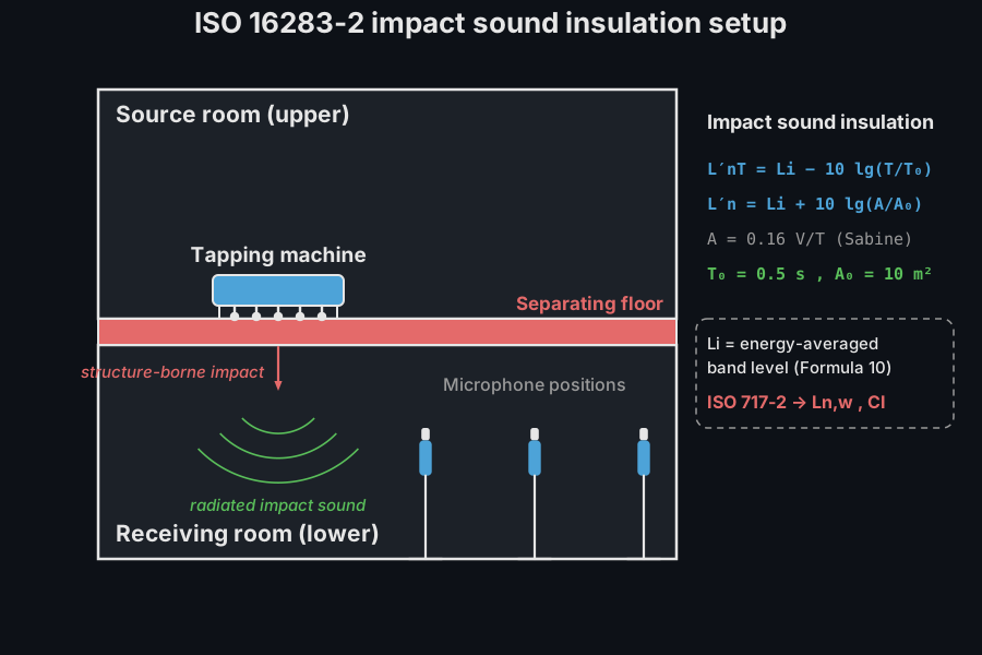
Section titled “Field impact insulation (ISO 16283-2)”Footstep noise is rated the other way round. Instead of how much a floor blocks, impact insulation measures how much a standardized tapping machine on the floor above puts into the room below, so a higher number is worse. The energy-average impact sound pressure level in the receiving room is normalised like the airborne case, but with a sign flip on the reverberation term:
The standardized impact level ( s for dwellings) needs only the receiving-room , so with s it equals ; the normalized level (referenced to a 10 m² absorption area) also needs the receiving-room volume. Note the minus sign: more reverberation lowers , opposite to the airborne .
The tapping machine is not the only source ISO 16283-2 specifies. Its hammers deliver a hard, quasi-stationary excitation whose energy sits above 100 Hz, which says almost nothing about the slow low-frequency thumps occupants actually complain about: a child jumping, an adult walking barefoot. For those, the same standard specifies a rubber ball (Annex A), rated through a different engine entirely: a Fast-weighted maximum level and the A-weighted sum of ISO 717-2 Annex D, not a shifted reference curve. It has its own guide, Heavy and Soft Impact Sources.
import numpy as npfrom phonometry import building
# 16 one-third-octave impact levels Li (100 Hz - 3150 Hz), dB, from the# ISO 717-2 Annex C worked example, and the receiving-room T per band.li = np.array([62.1, 63.2, 63.5, 66.2, 68.5, 70.0, 71.7, 73.1,               73.8, 73.5, 73.8, 73.3, 73.1, 73.0, 72.4, 71.2])t2 = np.full(16, 0.5)
imp = building.impact_insulation(li, t2, volume=50.0)print(round(float(imp.l_n_t[0]), 1))          # 62.1  (= Li since T = T0)print(round(float(imp.l_n[0]), 1))            # 64.1  normalized to A0 = 10 m^2
# Weighted impact rating + spectrum adaptation term CI (ISO 717-2)res_imp = building.weighted_impact_rating(imp.l_n_t)print(res_imp.rating, res_imp.ci, res_imp.unfavourable_sum)   # 79 -11 28.0  ->  L'nT,w(CI)=79(-11)
# Octave-band data carry the extra -5 dB reduction (Clause 4.3.2)octave = np.array([65.3, 64.5, 58.0, 55.8, 43.0])print(building.weighted_impact_rating(octave).rating)  # 54
Feed impact_insulation’s l_n_t (or l_n) straight into
weighted_impact_rating; the rating and reproduce the ISO 717-2 Annex C
values (thirds , ; octave 54, ).
The sign of the scale reverses here: lower is better for an impact quantity. National limits for dwellings sit in the 50 to 60 dB range, so dB is a bare structural floor with no covering and no floating layer, failing by roughly 20 dB. The Annex C example is a worst case, not a typical one. What it takes to close a gap of that size is a floating floor on a resilient layer or a decoupled ceiling, not a carpet; see Predicting Sound Insulation (EN 12354) and Predicting resilient-layer performance.
impact_insulation() parameters
Section titled “impact_insulation() parameters”| Parameter | Type | Units | Range / default | Notes |
|---|---|---|---|---|
li | 1D or 2D array | dB | one/band, or (positions, bands) | Energy-average impact SPL (2D is averaged over positions) |
t2 | 1D array | s | > 0, one per band | Receiving-room reverberation time |
volume | float, optional | m³ | > 0 | Receiving-room (enables ) |
t0 | float | s | default 0.5 | Reference reverberation time |
impact_insulation() returns an ImpactInsulationResult (l_n_t, l_n or
None); the ISO 717-2 side of the chain is in
Insulation Ratings (ISO 717).
ISO 16283 field test report (.report())
Section titled “ISO 16283 field test report (.report())”The per-band field results write the test report of ISO 16283-1:2014 /
ISO 16283-2:2020 Clause 14 directly, laid out like the recommended results
forms (Annex B / Annex C) and the accredited field reports built on them.
AirborneInsulationResult.report() renders the standardized level difference
fiche (Figure B.1) or, with quantity="r_prime", the apparent sound
reduction index fiche (Figure B.2); ImpactInsulationResult.report()
renders the standardized fiche (Figure C.1) or, with
quantity="l_n", the normalized fiche (Figure C.2). Each fiche names
the field standard in its basis line, evaluates the ISO 717-1 / ISO 717-2
single-number rating over the 16 core one-third-octave bands (100–3150 Hz),
states the quantity to one decimal place both in tabular form and as a curve
against the shifted reference curve (Clause 12), boxes the field rating
(DnT,w (C; Ctr), R'w (C; Ctr), L'nT,w (CI) or L'n,w (CI)) and prints
the mandatory statement that the evaluation is based on field measurement
results obtained by an engineering method.
verbose=True swaps the two-column table for the per-band measurement chain
(the energy-average and , or , and the reverberation time
beside the reported quantity), the content accredited field reports annex;
it needs a result built by airborne_insulation() / impact_insulation(),
which retain those inputs on the result (l1, l2/li, t2, t0).
Metadata, the requirement verdict (airborne passes at or above it, impact at
or below it), language="es" and the phonometry[report] extra behave
exactly as in the ISO 717 fiche above.
import numpy as npfrom phonometry import building, ReportMetadata
# Field airborne: source/receiving levels and T per one-third-octave bandl1 = np.array([92.3, 93.1, 94.0, 94.4, 94.8, 95.0, 95.2, 95.4,               95.3, 95.1, 94.8, 94.4, 93.9, 93.3, 92.5, 91.6])l2 = l1 - np.array([38.2, 40.1, 42.6, 45.2, 47.8, 50.1, 52.3, 54.0,                    55.6, 57.1, 58.2, 59.0, 59.6, 60.1, 60.3, 59.8])t2 = np.array([0.62, 0.58, 0.55, 0.53, 0.52, 0.50, 0.49, 0.48,               0.47, 0.46, 0.45, 0.45, 0.44, 0.43, 0.43, 0.42])field = building.airborne_insulation(l1, l2, t2, area=12.5, volume=30.4)field.plot()   # per-band DnT (and R') of the measured chain (needs matplotlib)metadata = ReportMetadata(    specimen="Separating wall, 240 mm brick with independent lining",    client="Example client",    area=12.5, source_volume=32.1, receiving_volume=30.4,    test_room="Dwelling A living room to dwelling B living room",    test_date="2026-07-20",    laboratory="Phonometry Reference Laboratory",    report_id="PHN-2026-0143",    requirement=50.0,               # DnT,w >= 50 dB -> PASS/FAIL row)field.report("DnTw_field.pdf", metadata=metadata)      # DnT,w (C; Ctr)field.report("Rpw_field.pdf", quantity="r_prime",             metadata=metadata)                        # R'w (C; Ctr)field.report("DnTw_chain.pdf", metadata=metadata,             verbose=True)                             # f | L1 | L2 | T | DnT
# Field impact: tapping-machine levels in the receiving roomli = np.array([58.0, 60.5, 62.0, 63.5, 65.0, 66.0, 66.5, 66.0,               65.5, 65.0, 64.0, 62.0, 59.0, 56.0, 53.0, 50.0])imp = building.impact_insulation(li, t2, volume=30.4)imp.report("LnTw_field.pdf",           metadata=ReportMetadata(requirement=58.0))  # L'nT,w (CI)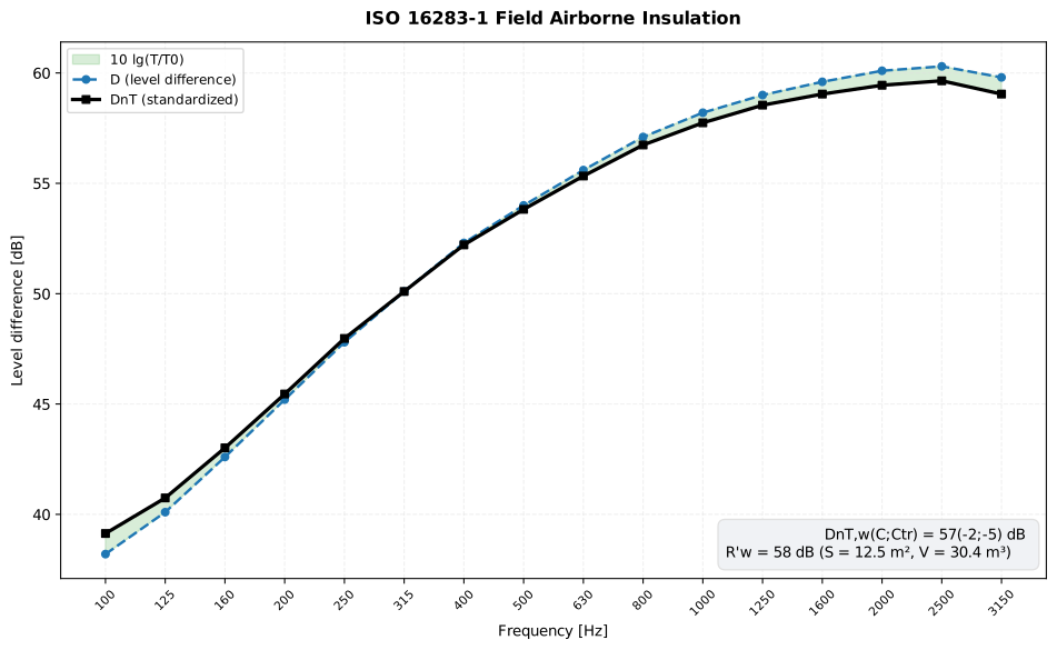
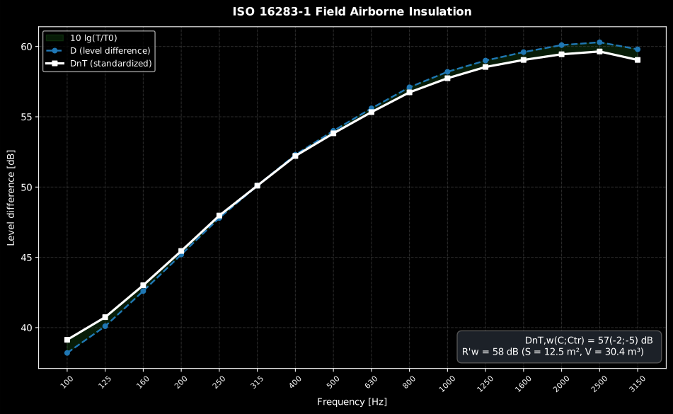
The receiving-room reverberation time turns the raw level difference into the standardized band by band; with above s across the range, the correction lifts the curve slightly. The rating box carries both single numbers of this measurement, and .
Show the code for this figure
import matplotlib.pyplot as pltimport numpy as npfrom phonometry import building
# Field airborne: source/receiving levels and T per one-third-octave bandl1 = np.array([92.3, 93.1, 94.0, 94.4, 94.8, 95.0, 95.2, 95.4,               95.3, 95.1, 94.8, 94.4, 93.9, 93.3, 92.5, 91.6])l2 = l1 - np.array([38.2, 40.1, 42.6, 45.2, 47.8, 50.1, 52.3, 54.0,                    55.6, 57.1, 58.2, 59.0, 59.6, 60.1, 60.3, 59.8])t2 = np.array([0.62, 0.58, 0.55, 0.53, 0.52, 0.50, 0.49, 0.48,               0.47, 0.46, 0.45, 0.45, 0.44, 0.43, 0.43, 0.42])field = building.airborne_insulation(l1, l2, t2, area=12.5, volume=30.4)
# One line — the per-band DnT (and R') of the measured chain:field.plot()plt.show()
# By hand, from the result's fields:bands = [100, 125, 160, 200, 250, 315, 400, 500,         630, 800, 1000, 1250, 1600, 2000, 2500, 3150]x = np.arange(len(bands))w = building.weighted_rating(field.dnt)fig, ax = plt.subplots()ax.fill_between(x, field.d, field.dnt, alpha=0.2, label="10 log10(T/T0)")ax.plot(x, field.d, "--o", label="D (level difference)")ax.plot(x, field.dnt, "-s", label="DnT (standardized)")ax.set_xticks(x, [str(b) for b in bands], rotation=45)ax.set(xlabel="Frequency [Hz]", ylabel="Level difference [dB]",       title=f"DnT,w = {w.rating} dB  (C={w.c:+d}; Ctr={w.ctr:+d})")ax.legend()plt.show()
Both example fiches are regenerated with make reports and kept rendered in
the repository; click either preview to open the PDF.
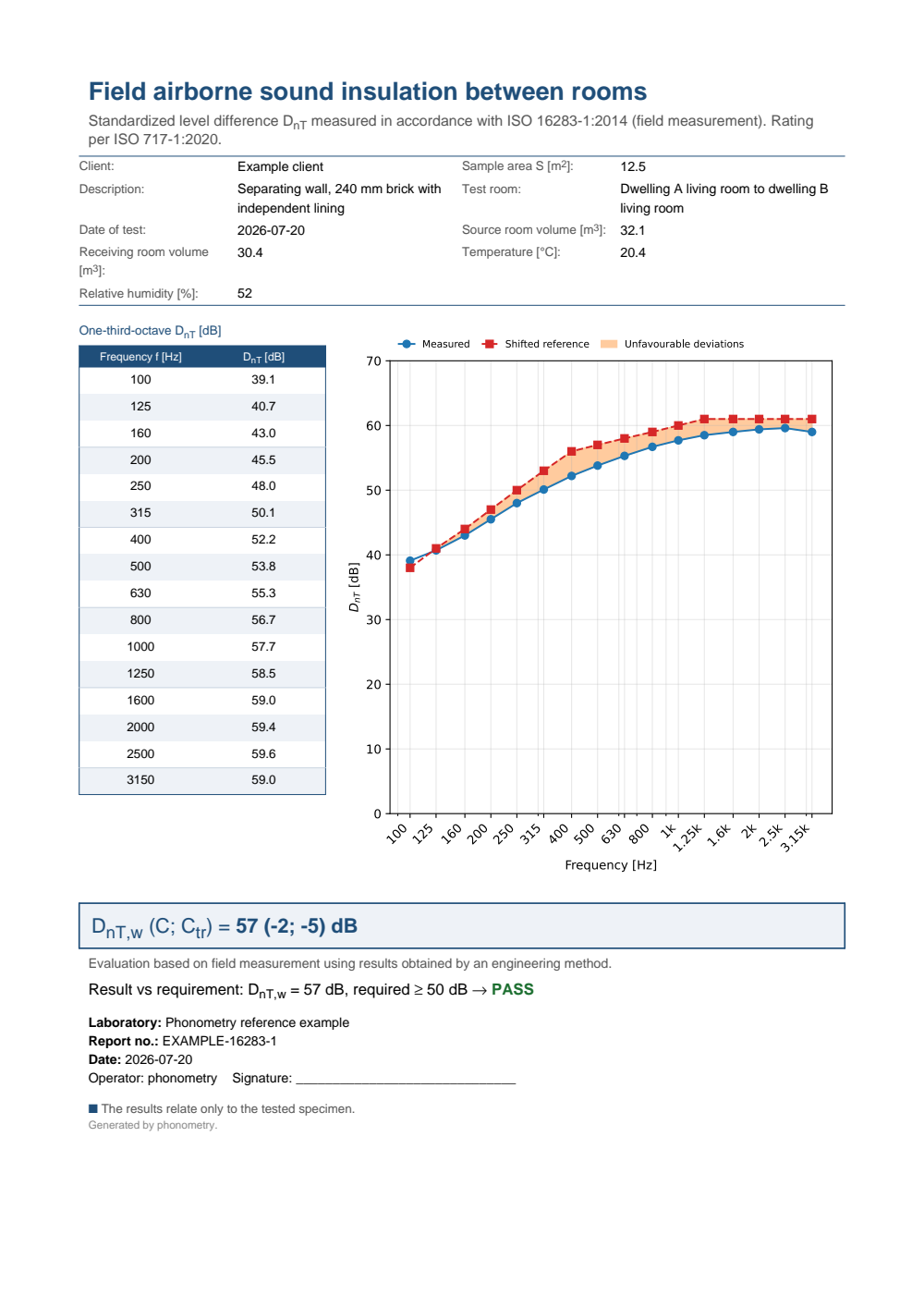
One-page field airborne sound insulation test report between dwellings: the metadata header (client, construction description, partition area, room volumes, climate), the one-third-octave DnT table beside the measured-versus-shifted-reference curve, the boxed DnT,w (C; Ctr) field rating, the engineering-method statement and a PASS verdict against the 50 dB requirement.
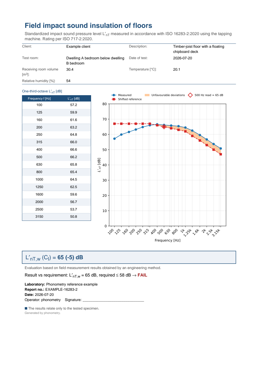
One-page field impact sound insulation test report for a floor under tapping-machine excitation: the metadata header, the one-third-octave L'nT table beside the measured-versus-shifted-reference curve with the 500 Hz read-off, the boxed L'nT,w (CI) field rating, the engineering-method statement and a FAIL verdict against the 58 dB requirement (a lower impact level is better).
Measurement uncertainty (ISO 12999-1)
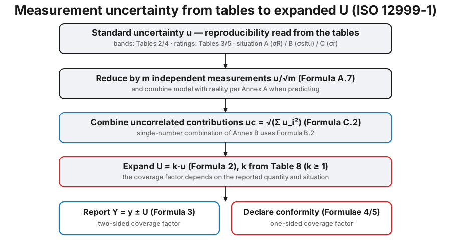
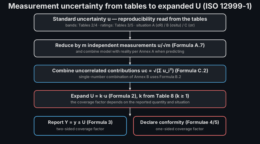
Section titled “Measurement uncertainty (ISO 12999-1)”A rating without an uncertainty is only half a result. ISO 12999-1 does not re-measure anything; it tabulates the standard uncertainty of every sound-insulation quantity, derived from inter-laboratory tests, and prescribes how to expand and combine it. Which standard deviation is depends on the measurement situation (Clause 5.2):
| Situation | Meaning | Standard uncertainty |
|---|---|---|
| A | laboratory characterisation (ISO 10140) | reproducibility |
| B | same location, different teams | in-situ |
| C | same location, same operator repeated | repeatability |
The expanded uncertainty is (Formula 2) with the coverage factor of Table 8. A two-sided interval (Formula 3, at 95 %) reports a value; the one-sided factor ( at 95 %) declares conformity with a requirement (Formulae 4/5).
from phonometry import building
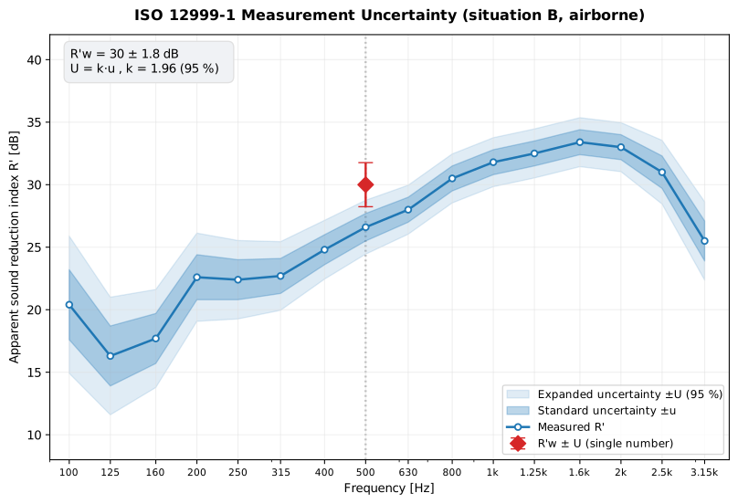
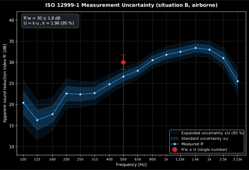
# Situation B (same building, different teams) -> the in-situ standard deviation.print(building.single_number_uncertainty("r_w", "B"))       # 0.9  dB  (Table 3)u = building.band_uncertainty("airborne", "B")              # per-band u (Table 2)# Look the band up; never index by position. The impact table has no 500 Hz# band at all, so [10] would silently be 630 Hz there.i = list(u.frequencies).index(500.0)print(len(u.frequencies), u.uncertainties[i])      # 21 1.1  (the 500 Hz band)u.plot()   # the per-band u(f) spectrum of Table 2 (needs matplotlib)
# Report R'w = 52 dB with a two-sided 95 % interval (k = 1.96, Table 8):uv = building.uncertain_value(52.0, "rprime_w", "B")        # aliases resolve to r_wprint(uv.coverage_factor, round(uv.expanded_uncertainty, 1))    # 1.96 1.8print(round(uv.lower, 1), round(uv.upper, 1))      # 50.2 53.8  ->  52 ± 1.8 dB
# Declaring conformity uses the ONE-sided factor (k = 1.65): does R'w provably# clear a 50 dB requirement?uc = building.uncertain_value(52.0, "rprime_w", "B", one_sided=True)print(round(uc.expanded_uncertainty, 2))                # 1.48  = 1.65 x 0.9print(round(52.0 - uc.expanded_uncertainty, 2))         # 50.52 = the lower boundprint(building.satisfies_lower_requirement(52.0, uc.expanded_uncertainty, 50.0))   # True
That is the whole content of satisfies_lower_requirement: the measured 52.0
minus the one-sided expanded uncertainty 1.48 is 50.52, which still clears
50.0, so conformity can be declared rather than merely observed. The choice
of factor is the point. Reporting a value is a two-sided statement (the true
value lies somewhere in an interval) and takes k = 1.96. Declaring
conformity is a one-sided statement: only the lower end matters, because
nothing is at stake if the wall is better than claimed, so k = 1.65 gives the
same 95 % confidence on the side that counts. Using the two-sided factor here
would demand 1.76 dB of margin instead of 1.48 dB and would fail results that
genuinely comply.
Impact quantities offer situations B/C only (Table 4, no 500 Hz band in the 2020
edition), and only situation A. Descriptors are case-insensitive with
aliases (rprime_w/dnt_w→r_w, lprime_n_w→ln_w); combine independent
components in quadrature with combine_uncertainties, and reduce by
independent measurements with reduce_by_independent_measurements ().
The same rating, reported three ways. Which interval applies is not a property of the measurement but of the question: situation A is what a laboratory quotes for a specimen, B what two teams measuring the same installed partition should agree within, C what one team repeating itself should. B is the widest of the three that a field report can honestly claim, and it is the one that decides whether a result clears a requirement.
Show the code for this figure
import matplotlib.pyplot as pltfrom phonometry import building
# The same R'w = 52 dB reported in each situation with its two-sided 95 % U.situations = ["A", "B", "C"]vals = [building.uncertain_value(52.0, "r_w", s) for s in situations]
fig, ax = plt.subplots(figsize=(7, 4))ax.errorbar(situations, [v.value for v in vals],            yerr=[v.expanded_uncertainty for v in vals],            fmt="o", capsize=8, color="tab:blue")for s, v in zip(situations, vals):    ax.annotate(f"±{v.expanded_uncertainty:.1f}", (s, v.upper),                textcoords="offset points", xytext=(8, 4))ax.set_ylabel("R'w [dB]"); ax.set_xlabel("Measurement situation")ax.set_title("R'w = 52 dB with 95 % expanded uncertainty (ISO 12999-1)")fig.tight_layout()plt.show()
band_uncertainty() / single_number_uncertainty() / uncertain_value() parameters
Section titled “band_uncertainty() / single_number_uncertainty() / uncertain_value() parameters”| Parameter | Type | Units | Range / default | Notes |
|---|---|---|---|---|
measurand | str | — | 'airborne' / 'impact' / 'impact_reduction' | Selects Table 2 / 4 / 6 |
quantity | str | — | 'r_w', 'ln_w', 'delta_lw' (+ aliases, +c/+ctr variants) | Single-number descriptor |
situation | str | — | 'A' / 'B' / 'C' | Measurement situation (Clause 5.2) |
value | float | dB | — | Best estimate to attach to |
coverage | float | — | default 0.95 | Confidence level (Table 8) |
one_sided | bool | — | default False | One-sided factor for conformity checks |
upper_limit | bool | — | default False | Select the upper limit (airborne, situation A) |
band_uncertainty() returns a BandUncertainty (frequencies,
uncertainties, .to_arrays()); single_number_uncertainty() a float;
uncertain_value() an UncertainValue (value, standard_uncertainty,
coverage_factor, expanded_uncertainty, .lower, .upper). The read-only
COVERAGE_FACTORS mapping exposes Table 8 keyed by (confidence, one_sided).
Beyond the two-room measurement
Section titled “Beyond the two-room measurement”Three neighbouring measurements have guides of their own, and a fourth sits alongside them. The building envelope, measured against the level 2 m in front of it and predicted from its elements, is Façade Sound Insulation. When a full engineering measurement is more than the question deserves, the octave-band control method is Sound Insulation Survey Method (ISO 10052). Every single number quoted above comes from the reference curves of Insulation Ratings (ISO 717). And the sound-intensity route to the same quantities, which reads the transmitted power off the radiating face instead of the receiving-room level, is Sound Insulation by Intensity (ISO 15186).
What this guide covers
Section titled “What this guide covers”Covered
ISO 16283-1:2014 (airborne field insulation: the level difference, standardized and apparent of Clause 3.12-3.15 and the Clause 7.8 position averaging) and ISO 16283-2:2020 (impact field insulation, the same normalisations with the sign flip) through
building.energy_average_level,building.airborne_insulationandbuilding.impact_insulation, each writing the Clause 14 test report with.report(); and ISO 12999-1:2020’s tabulated standard uncertainties (the Clause 5.2 measurement situations A/B/C and the Table 8 coverage factors, one- and two-sided) viabuilding.band_uncertainty,building.single_number_uncertaintyandbuilding.uncertain_value. The single-number ratings quoted here reuse the verified ISO 717-1/ISO 717-2 engines.Not covered
Every field function here takes levels that the caller has already corrected for background noise (Clause 9.2 of ISO 16283-1). The measurement of the background level (source off, same positions, same averaging) is the operator’s job, and nothing here verifies that the 6 dB floor was met; the correction itself is three lines of NumPy, written out under Correcting for background noise above. (
building.background_correctionis the ISO 10140-4 laboratory variant and does not match the field thresholds.) ISO 16283-1/-2’s own position requirements (the counts, distances and placements of Taking the measurement) are documented here and checked nowhere: energy-averaging happens once positions are supplied, but nothing verifies how many were taken or where. The low-frequency procedure of Small rooms is implemented: the 25 m³ trigger, Formula (12), Formula (13) and the 63 Hz octave reverberation time of Clause 10.4, but it too is fed corner levels the operator measured, and the only sampling requirement it enforces is a warning below the four corners per source position Clause 8.3 asks for. The other members of the family are covered by their own guides: the façade part ISO 16283-3 (Façade Sound Insulation), the survey method ISO 10052 (Sound Insulation Survey Method), the rating engines ISO 717-1/-2 (Insulation Ratings) and the sound-intensity route ISO 15186-1/-2 (Sound Insulation by Intensity).
Quick answers
Section titled “Quick answers”What does DnT,w mean?
Section titled “What does DnT,w mean?”is the weighted standardized level difference. Per one-third-octave band, references the receiving-room reverberation time to s, with the source-to-receiving level difference (ISO 16283-1). The ISO 717-1 reference-curve method then collapses the 16 bands from 100 Hz to 3150 Hz into the single number read at 500 Hz.
What is the difference between R and R’ in sound insulation?
Section titled “What is the difference between R and R’ in sound insulation?”The prime marks where the measurement was made: primed quantities (, , ) are measured in the building and include every flanking path, while the unprimed and are laboratory properties of the element alone, measured with flanking suppressed. In the field (ISO 16283-1), with partition area and Sabine absorption area .
References
Section titled “References”- Hopkins, C. (2007). Sound insulation. Butterworth-Heinemann. https://doi.org/10.4324/9780080550473The comprehensive treatment of airborne and impact sound insulation: the measurement chains, the statistics of rooms behind the field quantities and the interpretation of the single-number ratings. ISBN 978-0-7506-6526-1.
- International Organization for Standardization. (2014). Acoustics — Field measurement of sound insulation in buildings and of building elements — Part 1: Airborne sound insulation (ISO 16283-1:2014). The field airborne method this page implements: the level differences and normalisations.
- International Organization for Standardization. (2020). Acoustics — Determination and application of measurement uncertainties in building acoustics — Part 1: Sound insulation (ISO 12999-1:2020). The standard uncertainties per measurement situation (Clause 5.2) and the Table 8 coverage factors; its precision framework builds on ISO 5725 (context, not implemented directly).
- International Organization for Standardization. (2020). Acoustics — Field measurement of sound insulation in buildings and of building elements — Part 2: Impact sound insulation (ISO 16283-2:2020). The field impact method: the standardized and normalized impact levels, the Clause 14 test report and its Annex C results forms. The 2015 first edition is identical for the normalisations used here.
- International Organization for Standardization. (2020). Acoustics — Rating of sound insulation in buildings and of building elements — Part 1: Airborne sound insulation (ISO 717-1:2020). The reference-curve rating and the spectrum adaptation terms C and Ctr interpreted above; also the single-number engine for the façade quantity (Annex F).
- International Organization for Standardization. (2020). Acoustics — Rating of sound insulation in buildings and of building elements — Part 2: Impact sound insulation (ISO 717-2:2020). The impact reference-curve rating and the spectrum adaptation term CI, with the enlarged-range CI,50-2500 term.
- Vigran, T. E. (2008). Building acoustics. CRC Press. https://doi.org/10.1201/9781482266016A compact textbook companion for the sound-transmission physics behind these measurements. ISBN 978-0-415-42853-8.