Predicting Panel Sound Insulation

A laboratory test measures the sound reduction index $R$ of a finished element; this page instead predicts $R(f)$ from the physical properties of the construction, so a partition can be designed before it is built. It covers the airborne insulation of a single panel (the mass law and the coincidence dip), the double wall (its mass-spring-mass resonance), the transmission through slits and apertures that caps any real construction, the radiation efficiency of a bending plate, and the point mobilities that set the vibrational power a structure absorbs. Beside those it carries three shortcuts and special cases the same sources give: the plateau method, a hand estimate of a single panel’s whole curve from a table of materials (Norton 3.9.1); the orthotropic panel, where a corrugated or ribbed sheet has two critical frequencies and therefore a coincidence range instead of a dip (Vigran 6.5.3); and the wall-tie bridge that limits a masonry cavity wall whatever its leaves are worth (Hopkins 4.3.5.4). The measured counterparts these predictions feed live in Predicting Sound Insulation (EN 12354) and Field Insulation Measurement (ISO 16283).

A note on two symbols before the formulae start. The sound reduction index $R$ of the European standards and the transmission loss $TL$ of the North American literature this page follows are the same quantity, $TL\equiv R=-10\lg \tau$; the page keeps each source’s own symbol so its formulae can be checked against the printed text, which is why the results expose transmission_loss and rate it as $R_w$. Likewise, this page writes the mass per unit area $m^{\prime \prime }$, which is Bies’s and Hopkins’s notation for the $m^{\prime }$ used throughout the ISO 12354 guides; $m$ alone is reserved elsewhere on the site for the air power-attenuation coefficient of the reverberation formulae, in 1/m.

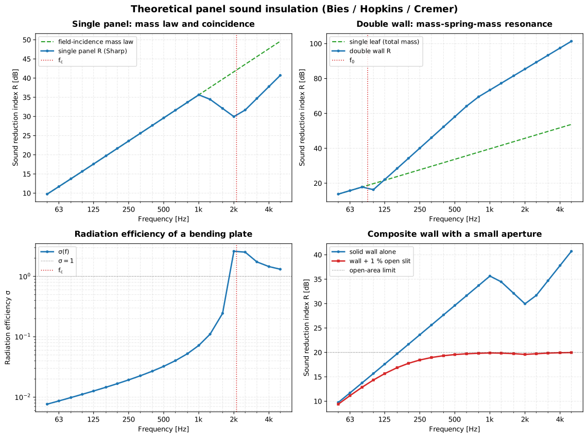
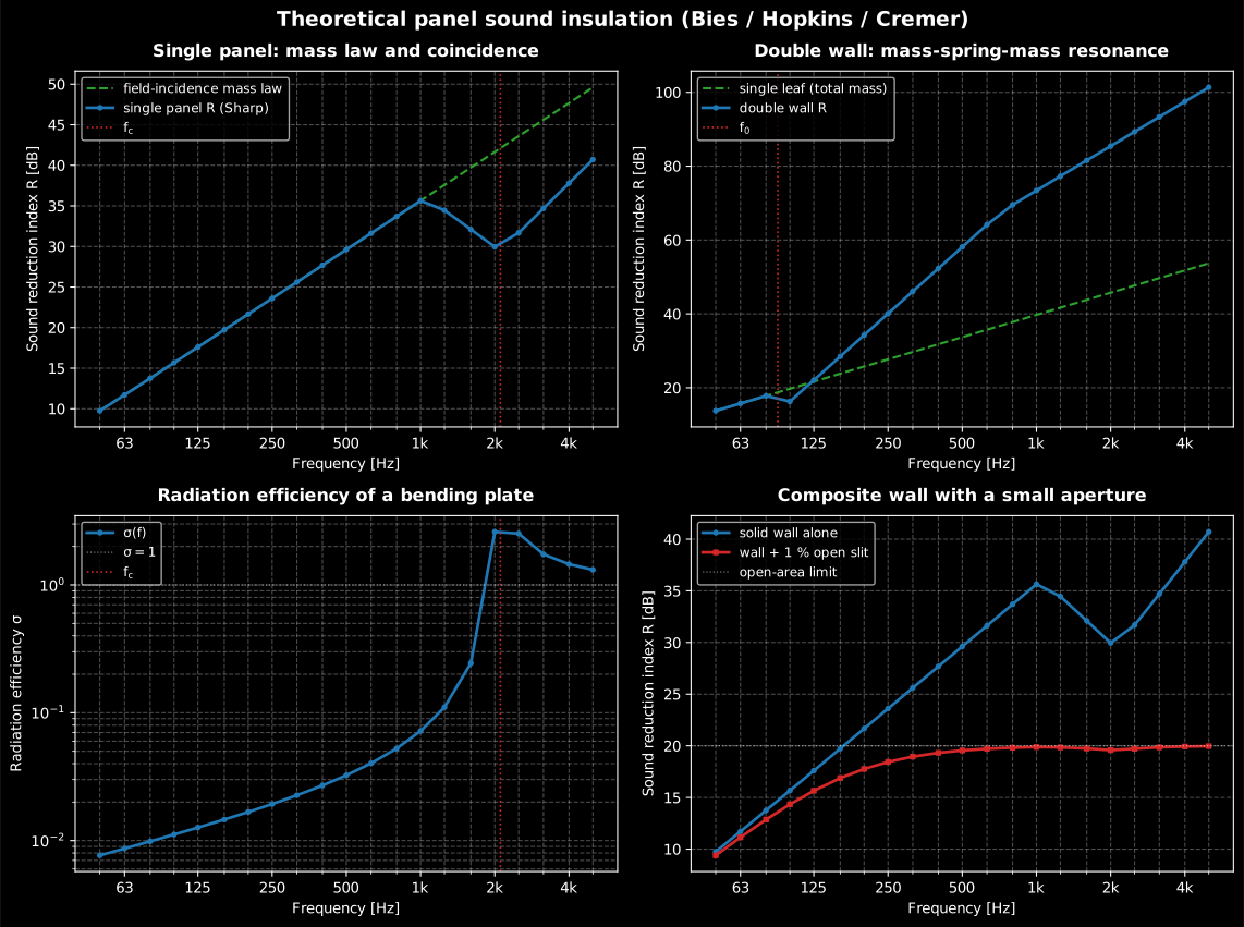
The four models of this page as a map, each panel a section below. Top left, the single leaf: 6 dB per octave until Sharp’s coincidence dip, 11.9 dB under the mass law in the 2.5 kHz band. Top right, splitting the same 24 kg/m² in two: 3.4 dB worse than one leaf at the 89 Hz mass-spring resonance and 47.7 dB better at 5 kHz. Bottom left, radiation efficiency: 0.011 at 100 Hz, 2.61 at coincidence, and only slowly back towards 1. Bottom right, the leak that ends the argument — 1 % of the area left open holds $R$ at 20.0 dB no matter what the wall is worth.

Show the code for the concept figure

import numpy as np
import matplotlib.pyplot as plt
from phonometry import (
    coincidence_frequency, composite_transmission_loss,
    double_wall_transmission_loss, mass_law_transmission_loss,
    mass_spring_mass_resonance, plate_bending_stiffness,
    radiation_efficiency, single_panel_transmission_loss,
)

bands = np.array([50, 63, 80, 100, 125, 160, 200, 250, 315, 400, 500, 630, 800,
                  1000, 1250, 1600, 2000, 2500, 3150, 4000, 5000], dtype=float)
fig, ax = plt.subplots(2, 2, figsize=(12, 9))

bp = plate_bending_stiffness(6.2e10, 0.006, 0.24)
fc = coincidence_frequency(15.0, bp)
ml = mass_law_transmission_loss(bands, 15.0, incidence="field")
sp = single_panel_transmission_loss(bands, 15.0, critical_frequency=fc, loss_factor=0.024)
ax[0, 0].semilogx(bands, ml, "--", label="field-incidence mass law")
ax[0, 0].semilogx(bands, sp.transmission_loss, "-o", ms=3, label="single panel R (Sharp)")
ax[0, 0].axvline(fc, ls=":", color="r"); ax[0, 0].set_title("Single panel")

dw = double_wall_transmission_loss(bands, 12.0, 12.0, 0.075)
ax[0, 1].semilogx(bands, mass_law_transmission_loss(bands, 24.0), "--", label="single leaf")
ax[0, 1].semilogx(bands, dw.transmission_loss, "-o", ms=3, label="double wall")
ax[0, 1].axvline(mass_spring_mass_resonance(12.0, 12.0, 0.075), ls=":", color="r")
ax[0, 1].set_title("Double wall")

sig = radiation_efficiency(bands, 1.5, 1.25, fc)
ax[1, 0].loglog(bands, sig.radiation_efficiency, "-o", ms=3, label=r"$\sigma(f)$")
ax[1, 0].axhline(1.0, ls=":"); ax[1, 0].set_title("Radiation efficiency")

wall = sp.transmission_loss
comp = [float(composite_transmission_loss([0.99, 0.01], [w, 0.0])) for w in wall]
ax[1, 1].semilogx(bands, wall, "-o", ms=3, label="solid wall")
ax[1, 1].semilogx(bands, comp, "-s", ms=3, label="wall + 1 % slit")
ax[1, 1].axhline(20.0, ls=":"); ax[1, 1].set_title("Composite with aperture")

for a in ax.flat:
    a.set_xlabel("Frequency [Hz]"); a.legend(fontsize=8); a.grid(alpha=0.3)
fig.suptitle("Theoretical panel sound insulation")
fig.tight_layout(); plt.show()

Single panel: the mass law and coincidence (Bies 7.2)

A limp, non-stiff panel transmits sound by being driven bodily by the incident pressure; the heavier it is and the higher the frequency, the more it resists. The normal-incidence mass law (Bies Eq. 7.40) and its diffuse-field form (Eq. 7.42) are

$$T{L}_0=10{\log }_{10}\left[1+{\left(\frac{\pi f{m}^{\prime \prime }}{{\rho }_0{c}_0}\right)}^2\right],TL=T{L}_0-{\Delta }_{\text{band}},$$

with $m^{\prime \prime }$ the mass per unit area and ${\Delta }_{\text{band}}=5.5$ dB (one-third octave) or $4.0$ dB (octave). Above the argument’s knee the mass law rises 6 dB per octave and 6 dB per doubling of mass, the two facts every insulation calculation rests on.

A real panel is also stiff, so at the coincidence (critical) frequency (Bies Eq. 7.3)

$$f_c=\frac{c_0^2}{2\pi }\sqrt{\frac{m^{\prime \prime }}{B^{\prime }}}=\frac{0.55c_0^2}{c_{L}h},$$

the free bending wavelength matches the trace wavelength of the incident sound and the panel goes transparent: the coincidence dip. Sharp’s method holds the field-incidence mass law up to $f_c/2$, drops through a straight line in $\log f$, and from $f_c$ upward follows (Eq. 7.44) $TL=10{\log }_{10}[1+(\pi f{m}^{\prime \prime }/{\rho }_0{c}_0{)}^2]+10{\log }_{10}(2\eta f/\pi f_c)$ with the loss factor $\eta$. The dip sits at Bies design-chart point B, $TL=20{\log }_{10}(f_c{m}^{\prime \prime })+10{\log }_{10}\eta -44$.

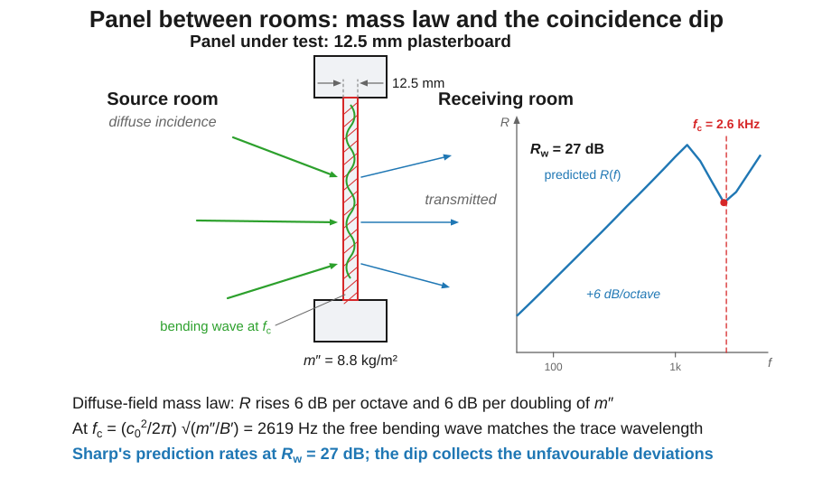
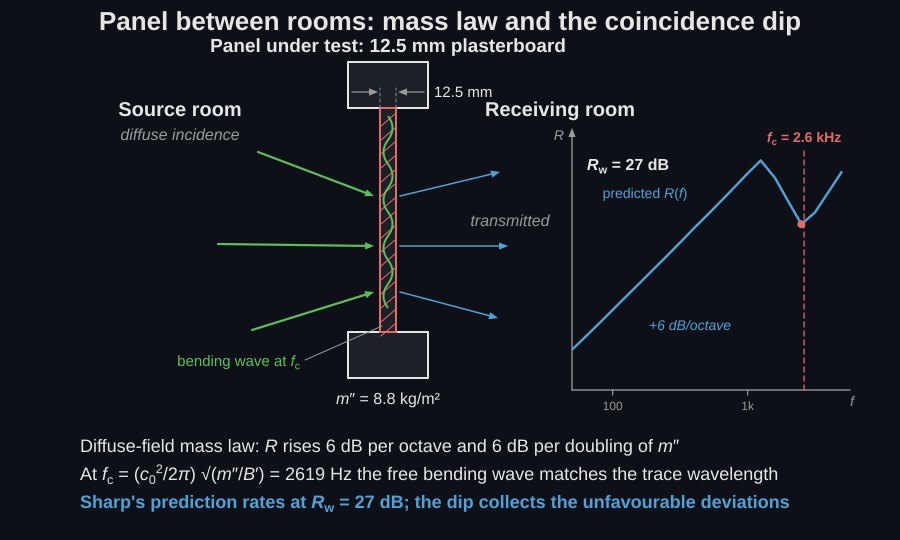
The whole section in one sketch: a diffuse field drives a single leaf, and the predicted $R(f)$ climbs with the mass law until the coincidence dip. A 12.5 mm plasterboard leaf puts $f_c$ near 2.6 kHz and rates $R_w=27$ dB.

import numpy as np
from phonometry import (
    coincidence_frequency, plate_bending_stiffness,
    single_panel_transmission_loss,
)

# 6 mm float glass: E = 62 GPa, rho = 2500 kg/m3, nu = 0.24, eta = 0.024.
bands = np.array([100, 125, 160, 200, 250, 315, 400, 500, 630, 800,
                  1000, 1250, 1600, 2000, 2500, 3150], dtype=float)
mass = 2500.0 * 0.006                                 # 15 kg/m2
bp = plate_bending_stiffness(6.2e10, 0.006, 0.24)     # B' [N.m]
fc = coincidence_frequency(mass, bp)
print(round(fc))                                      # 2107 Hz (Hopkins declares ~2079)

res = single_panel_transmission_loss(bands, mass, critical_frequency=fc,
                                     loss_factor=0.024)
print(round(res.rating().rating))                     # 32  ->  Rw = 32 dB (catalogue 6 mm glass)

res.plot()   # predicted R(f) with the critical frequency marked (needs matplotlib)

The predicted spectrum plugs straight into the ISO 717-1 rating through res.rating(), and into EN 12354 as the “predicted” element $R$ where the standard would otherwise demand a laboratory measurement.

Which loss factor is $\eta$? The total loss factor of the element as mounted, not the material’s internal loss factor. In a mounted element the total is internal plus radiation plus the losses at the edges, and for a heavy element in a test opening the edge term dominates: ISO 12354-1 Annex C gives ${\eta }_{\text{tot,lab}}\approx {\eta }_{\text{int}}+m^{\prime }/(485\sqrt{f})\approx 0,01+m^{\prime }/(485\sqrt{f})$ for elements below 800 kg/m², reachable without leaving the library as laboratory_total_loss_factor. For this 15 kg/m² pane that estimate is 0,011 at 500 Hz, barely above the internal value; for a 484 kg/m² concrete floor it is 0,055, five times the material figure. The measured route is the structural reverberation time and $\eta =2,2/(f{T}_s)$, the same quantity the ISO 10848 and EN 15657 guides measure. The stake is worth knowing: the dip depth carries $10\lg \eta$, so a factor of three in $\eta$ moves the coincidence region by 4,8 dB and changes nothing below $f_c/2$.

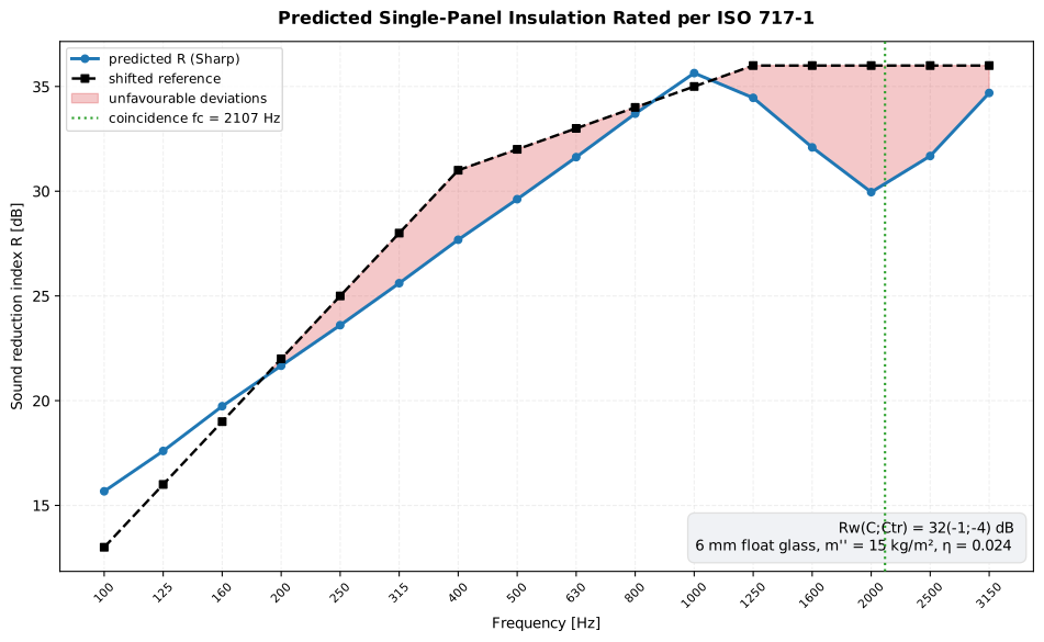
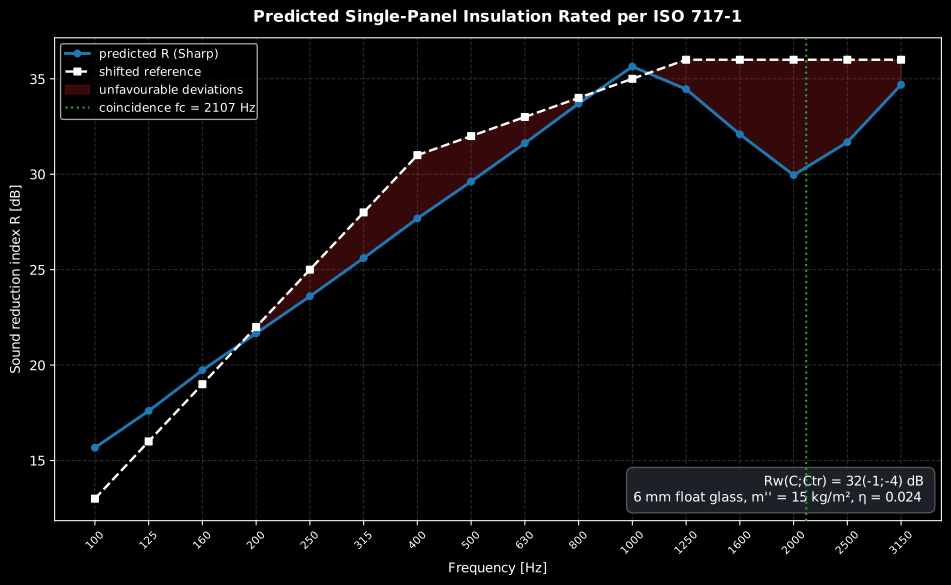
The predicted Sharp spectrum rated exactly like a measurement: the coincidence dip at $f_c\approx 2.1$ kHz collects most of the unfavourable deviations, and the shifted reference read at 500 Hz gives the catalogue $R_w=32$ dB of 6 mm glass.

Show the code for this figure

import matplotlib.pyplot as plt
import numpy as np
from phonometry import (
    coincidence_frequency, plate_bending_stiffness,
    single_panel_transmission_loss,
)

# 6 mm float glass: E = 62 GPa, rho = 2500 kg/m3, nu = 0.24, eta = 0.024.
bands = np.array([100, 125, 160, 200, 250, 315, 400, 500, 630, 800,
                  1000, 1250, 1600, 2000, 2500, 3150], dtype=float)
mass = 2500.0 * 0.006
bp = plate_bending_stiffness(6.2e10, 0.006, 0.24)
fc = coincidence_frequency(mass, bp)
res = single_panel_transmission_loss(bands, mass, critical_frequency=fc,
                                     loss_factor=0.024)
w = res.rating()

# One line each — the predicted R(f), or the rated curve vs the reference:
res.plot()
w.plot()
plt.show()

# By hand, combining both on one axes:
fig, ax = plt.subplots()
ax.semilogx(bands, res.transmission_loss, "o-", label="predicted R (Sharp)")
ax.semilogx(w.band_centers, w.shifted_reference, "s--",
            label="shifted reference")
ax.fill_between(w.band_centers, w.measured, w.shifted_reference,
                where=w.measured < w.shifted_reference, interpolate=True,
                alpha=0.3, label="unfavourable deviations")
ax.axvline(fc, ls=":", color="tab:green", label=f"fc = {fc:.0f} Hz")
ax.set_xlabel("Frequency [Hz]")
ax.set_ylabel(r"Sound reduction index $R$ (transmission loss $\mathrm{TL}$) [dB]")
ax.set_title(f"Rw = {w.rating} dB  (C={w.c:+d}; Ctr={w.ctr:+d})")
ax.legend()
plt.show()

The clip below watches coincidence happen in a 2D elastic FDTD field: a 10 mm steel plate immersed in air, driven by a sustained plane wave at 45 degrees, with both frequencies picked from the library’s coincidence_frequency. At fc/2 = 603 Hz the measured transmission lands on the oblique mass law; at 2 fc = 2413 Hz the 45-degree trace equals the bending wavelength exactly and the trace-matched plate re-radiates a 45-degree beam that grows along the plate, pinning the transmitted level at the fc/2 figure even though the mass law demands 12 dB more blocking at four times the frequency. The air drives the heavy steel so weakly that the resonant bending wave needs tens of metres of illuminated plate to build up fully, which is why a real coincidence dip, not total transparency, is what measurements show.

What the plate lets through is about 47 dB under the incident wave, so on the colour scale the standing wave above the plate sets, the transmitted field would be a black band. Both panels therefore draw the air below the plate with the display gain printed on them (x150, that is +44 dB); the gain is the same on the two so the panels stay comparable, and the level annotations are the measured, physical ones.

Two side-by-side elastic FDTD fields of the same 10 mm steel plate lying in air while a sustained plane wave arrives at 45 degrees. At 603 Hz, half the coincidence frequency, the wave reflects almost totally and the faint transmitted level matches the oblique mass law. At 2413 Hz, twice the coincidence frequency, the acoustic trace matches the free bending wavelength and a 45-degree transmitted beam grows below the plate, holding the same level as the low-frequency panel where the mass law predicted 12 dB more insulation, the air below the plate drawn on both panels with an annotated 150-fold display gain (+44 dB) so the transmitted field is legible, with the 1206 Hz coincidence frequency of the library and both measured and mass-law levels annotated.

Download the animation (WebM)

Two side-by-side elastic FDTD fields of the same 10 mm steel plate lying in air while a sustained plane wave arrives at 45 degrees. At 603 Hz, half the coincidence frequency, the wave reflects almost totally and the faint transmitted level matches the oblique mass law. At 2413 Hz, twice the coincidence frequency, the acoustic trace matches the free bending wavelength and a 45-degree transmitted beam grows below the plate, holding the same level as the low-frequency panel where the mass law predicted 12 dB more insulation, the air below the plate drawn on both panels with an annotated 150-fold display gain (+44 dB) so the transmitted field is legible, with the 1206 Hz coincidence frequency of the library and both measured and mass-law levels annotated.

Download the animation (WebM)

Quick estimates: the plateau method (Norton 3.9.1)

Before the physical model there is a shortcut that practitioners have drawn by hand for decades. The plateau method (Norton & Karczub 2003, Section 3.9.1, after Watters) approximates the whole field-incidence curve of a single panel from three numbers per material, tabulated in PLATEAU_MATERIALS from Norton’s Table 3.1: the surface density per millimetre of thickness, the height of the coincidence plateau in decibels, and the frequency ratio B/A that sets its width.

The construction has three parts:

1. the field-incidence mass law TL = 10 lg(1 + (π f m''/ρ₀c₀)²) − 5 dB (Norton Eqs. 3.104 and 3.106), rising 6 dB per octave;
2. a horizontal coincidence plateau at the tabulated height, with point A where the mass-law line reaches it;
3. point B at $B/A\times f_A$, above which the estimate recovers at 10 dB per octave.

It needs neither the bending stiffness nor the loss factor - the tabulated plateau absorbs both - and it assumes a diffuse field on both sides of a panel whose length and width are at least twenty times its thickness.

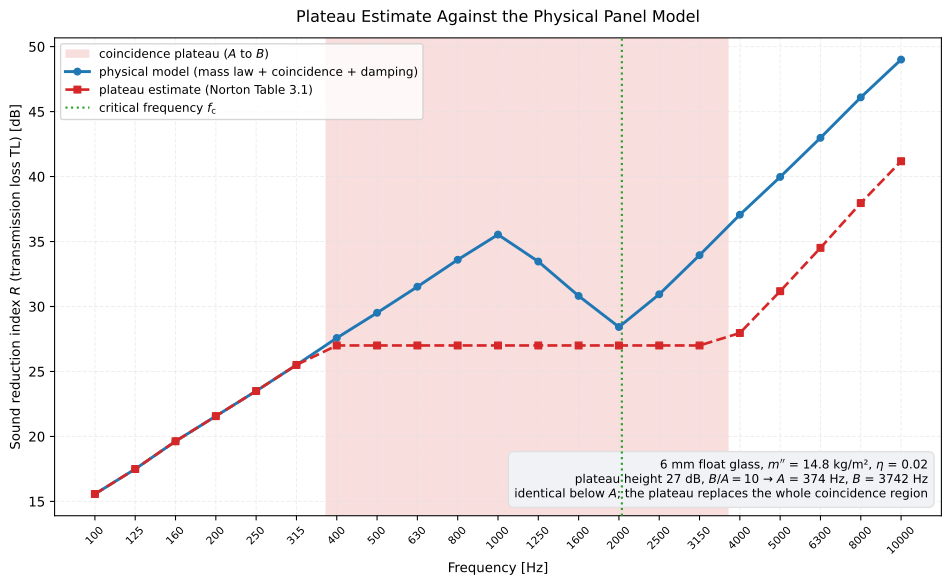
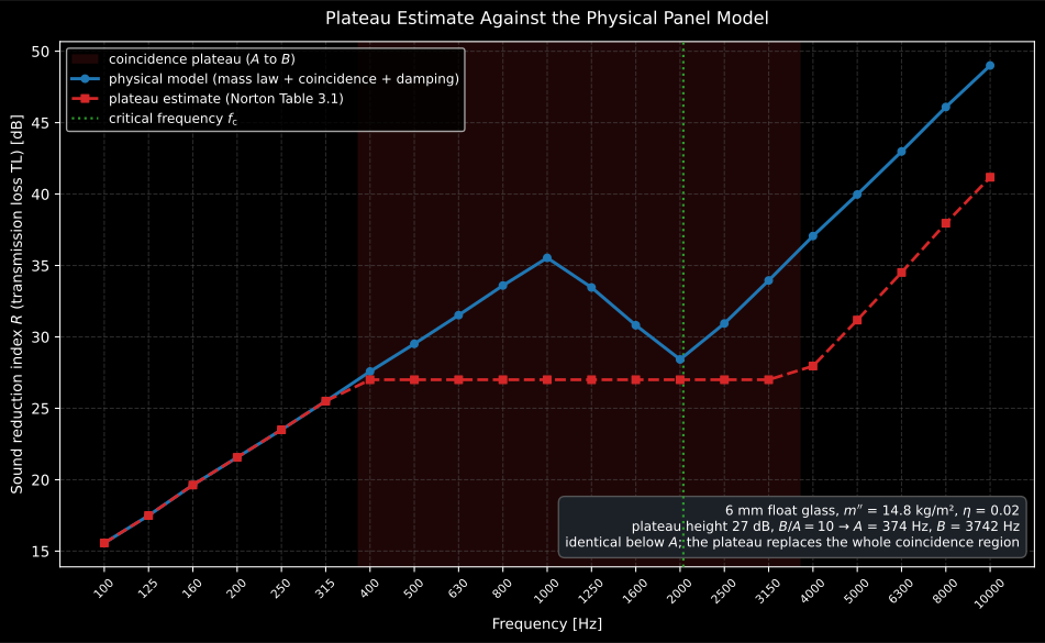
The two curves are the same line below point A. Above it the plateau estimate replaces the entire coincidence region with one flat value, which is exactly what it claims to be: an estimate, not the dip.

Show the code for this figure

import matplotlib.pyplot as plt
import numpy as np
from phonometry import plateau_transmission_loss, single_panel_transmission_loss

# 6 mm float glass: Norton Table 3.1 gives 2.47 kg/m2 per mm, a 27 dB
# coincidence plateau and B/A = 10; its critical frequency is 2033 Hz.
bands = np.array([100, 125, 160, 200, 250, 315, 400, 500, 630, 800, 1000,
                  1250, 1600, 2000, 2500, 3150, 4000, 5000, 6300, 8000,
                  10000], dtype=float)
quick = plateau_transmission_loss(bands, material="glass", thickness_mm=6.0,
                                  field_correction=5.5)
physical = single_panel_transmission_loss(bands, 2.47 * 6.0,
                                          critical_frequency=2033.0,
                                          loss_factor=0.02)

print(round(quick.plateau_start), round(quick.plateau_end))   # 374 3742
print(quick.plateau_height)                                   # 27.0
quick.plot()          # shades the plateau between points A and B
plt.show()

A worked check against the book: an 8 m x 3 m solid brick wall 110 mm thick at 2.1 kg/m² per mm ($m^{\prime \prime }=231{\text{kg/m}}^2$) gives 35.8 dB in the 63 Hz octave, on the mass-law line, then the brick plateau of 37 dB across the 125 Hz and 250 Hz octaves, then 10 dB per octave above point B - Norton’s printed answer to his problem 3.11 exactly, band for band, in the two regions the construction fixes analytically.

from phonometry import plateau_transmission_loss

octaves = [63.0, 125.0, 250.0, 500.0, 1000.0, 2000.0, 4000.0]
res = plateau_transmission_loss(octaves, material="brick", thickness_mm=110.0,
                                air_density=1.21)
print(res.transmission_loss.round(1))
# [35.8 37.  37.  43.3 53.3 63.3 73.3]

The physical model has its own Norton-flavoured variant for the region above coincidence: coincidence_model="cremer" replaces Sharp’s Eq. 7.44 with Cremer’s empirical TL = TL₀ + 10 lg(f/fc − 1) + 10 lg η − 2 dB (Norton Eq. 3.110), and runs the mass law right up to fc with no interpolated bridge. Both rise at about 10 dB per octave far above coincidence; they differ in how they leave the dip.

Orthotropic panels: a coincidence range, not a dip (Vigran 6.5.3)

Ribbed and corrugated cladding is not isotropic. It is very stiff along the corrugations and almost as limp as a flat sheet across them, so instead of one coincidence frequency it has a whole coincidence range bounded by the two principal bending stiffnesses (Vigran Eq. 6.107, the isotropic $f_c=(c_0^2/2\pi )\sqrt{m^{\prime \prime }/B}$ evaluated twice):

$$f_{c1}=\frac{c_0^2}{2\pi }\sqrt{\frac{m^{\prime \prime }}{B_1}},f_{c2}=\frac{c_0^2}{2\pi }\sqrt{\frac{m^{\prime \prime }}{B_2}},B_1>B_2.$$

The stiffest direction sets the lowest coincidence frequency, which is the sting in the tail: corrugating a sheet to gain strength drags $f_{c1}$ down, often to a few hundred hertz, while $f_{c2}$ runs up to 15 kHz or 30 kHz. Over that whole span the resonant transmission dominates and $R$ flattens far below the mass law of a flat plate of the same mass.

The bending-wave impedance now depends on the azimuth $\vartheta$ as well as the incidence angle $\phi$ (Heckl 1960; Hansen 1993; Vigran Eq. 6.108, which is Bies Eq. 7.30):

$$Z_w=\mathrm{j}\omega m^{\prime \prime }\left[1-{\left(\frac{f}{f_{c1}}{\cos }^2\vartheta +\frac{f}{f_{c2}}{\sin }^2\vartheta \right)}^2(1+\mathrm{j}\eta ){\sin }^4\phi \right],$$

and the diffuse-field average of $\tau =|1+Z_w\cos \phi /2{\rho }_0{c}_0{|}^{-2}$ becomes a double integral (Vigran Eq. 6.111 = Bies Eq. 7.38). Setting $f_{c1}=f_{c2}$ recovers Cremer’s isotropic impedance exactly.

orthotropic_transmission_loss offers both published routes:

• method="integral" evaluates that double integral numerically. It is the only route that responds to the loss factor, and it is the one that shows how deep the coincidence region really goes. The near-grazing angles are excluded by a limiting angle: pass area for the size-dependent limit of Bies Eq. 7.36 (Vigran writes it as Eq. 6.113), or leave it out for the fixed limiting_angle (78 degrees by default, Sharp’s value, which is Vigran’s ${\sin }^2\phi =0.96$).

• method="heckl" is Heckl’s closed-form approximation for $\eta =0$, the design chart of Bies Fig. 7.9(b): field-incidence mass law below $f_{c1}/2$, then

  $${\tau }_F\approx \frac{{\rho }_0{c}_0}{2{\pi }^2{m}^{\prime \prime }}\frac{f_{c1}}{f^2}{\left[\ln \frac{4f}{f_{c1}}\right]}^2(f_{c1}\le f<f_{c2}/2),{\tau }_F\approx \frac{{\rho }_0{c}_0}{2m^{\prime \prime }}\frac{\sqrt{f_{c1}{f}_{c2}}}{f^2}(f>2f_{c2}),$$

  with straight lines in ${\log }_{10}f$ across the two gaps. It needs no loss factor and no numerical work, but it requires $f_{c2}>4f_{c1}$ for its four construction points to stay in order.

For the common “wavy” corrugation the equivalent stiffnesses come from Timoshenko and Woinowsky-Krieger through corrugated_plate_stiffness (Vigran Eq. 3.115), and the surface density has to grow with the developed length of the profile, which is what corrugated_plate_mass_factor returns. orthotropic_plate_resonance is the matching eigenfrequency of a simply supported orthotropic plate (Vigran Eq. 3.113 = Bies Eq. 7.27, after Hearmon 1959); its lowest mode matters because both infinite-panel models are only valid above roughly $1.5f_{1,1}$.

from phonometry import (
    coincidence_frequency, corrugated_plate_mass_factor,
    corrugated_plate_stiffness, orthotropic_critical_frequencies,
    orthotropic_plate_resonance, plate_bending_stiffness,
)

# Vigran's worked example: a 1 m x 1 m steel sheet 1 mm thick, E = 210 GPa,
# nu = 0.3, m'' = 7.8 kg/m2, corrugated into a sinusoid 20 mm deep
# (amplitude H = 10 mm) at a 100 mm pitch.
flat_b = plate_bending_stiffness(2.1e11, 1.0e-3, 0.3)
b_x, b_z, b_xz = corrugated_plate_stiffness(
    1.0e-3, 0.010, 0.100, youngs_modulus=2.1e11, poisson_ratio=0.3,
)
mass = 7.8 * corrugated_plate_mass_factor(0.010, 0.100)
print(round(flat_b, 1), round(b_x, 1), round(b_z))     # 19.2 17.5 2202
print(round(mass, 2))                                  # 8.52 kg/m2 (+9 %)

flat = {"length_x": 1.0, "length_z": 1.0, "mass_per_area": 7.8,
        "bending_stiffness_x": flat_b, "bending_stiffness_z": flat_b,
        "bending_stiffness_xz": flat_b}
corr = {"length_x": 1.0, "length_z": 1.0, "mass_per_area": mass,
        "bending_stiffness_x": b_x, "bending_stiffness_z": b_z,
        "bending_stiffness_xz": b_xz}
print(round(orthotropic_plate_resonance(1, 1, **flat), 1),
      round(orthotropic_plate_resonance(2, 2, **flat), 1))    # 4.9 19.7
print(round(orthotropic_plate_resonance(1, 1, **corr), 1),
      round(orthotropic_plate_resonance(2, 2, **corr), 1))    # 25.5 102.1

# The same sheet, flat and corrugated, in the coincidence picture:
print(round(coincidence_frequency(7.8, flat_b)))               # 11925 Hz
print([round(f) for f in orthotropic_critical_frequencies(mass, b_x, b_z)])
# [1165, 13064]

The four eigenfrequencies are Vigran’s own printed answers (4.9 Hz, 19.7 Hz flat; 25.5 Hz, 102 Hz corrugated), and reproducing the corrugated pair is what proves the mass factor belongs there: with the flat 7.8 kg/m² the same formulas return 26.7 Hz and 106.7 Hz.

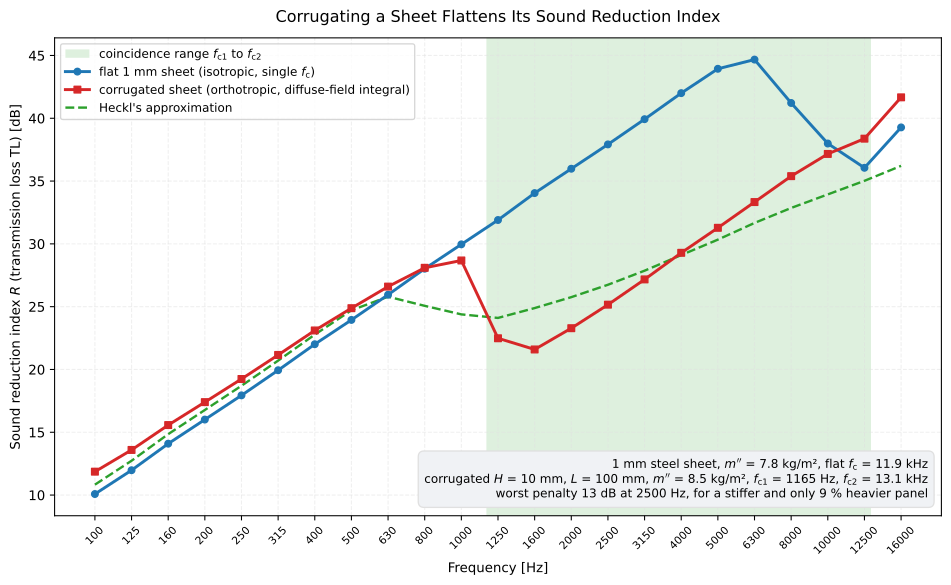
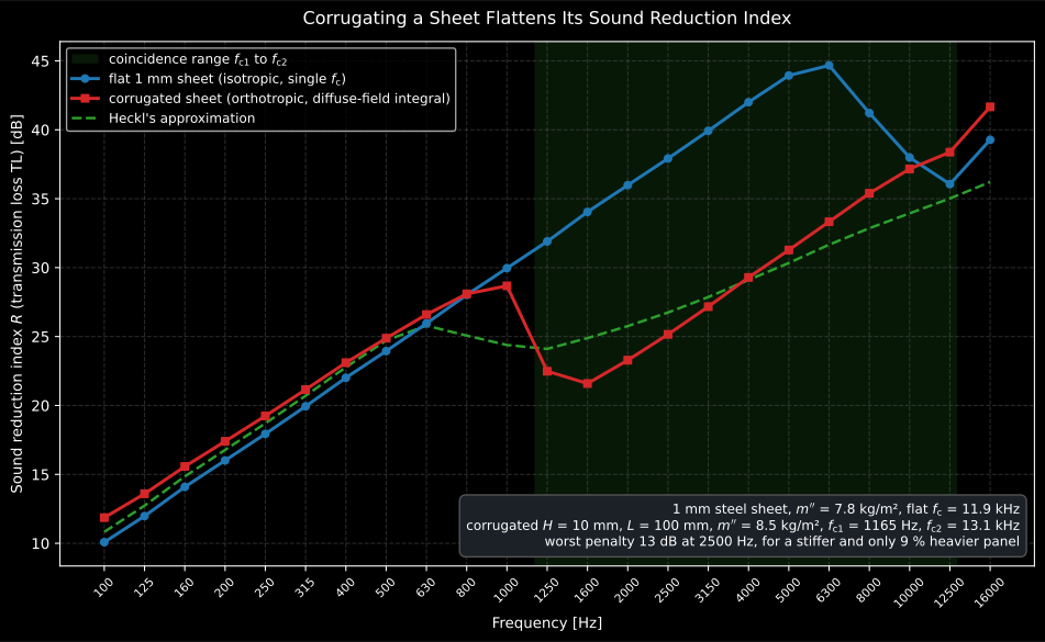
The trade corrugating makes, on Vigran’s own geometry. Below $f_{c1}$ the two panels are within about 2 dB of each other (the corrugated one slightly higher: it is 9 % heavier, and the diffuse-field integral uses a 78 degree limiting angle rather than Sharp’s 5.5 dB band correction). Across the coincidence range the corrugated sheet gives away up to 13 dB, and $R_w$ falls from 28 dB to 25 dB, for a panel that is stiffer and barely heavier.

Show the code for this figure

import matplotlib.pyplot as plt
import numpy as np
from phonometry import (
    coincidence_frequency, corrugated_plate_mass_factor,
    corrugated_plate_stiffness, orthotropic_critical_frequencies,
    orthotropic_transmission_loss, plate_bending_stiffness,
    single_panel_transmission_loss,
)

bands = np.array([100, 125, 160, 200, 250, 315, 400, 500, 630, 800, 1000,
                  1250, 1600, 2000, 2500, 3150, 4000, 5000, 6300, 8000,
                  10000, 12500, 16000], dtype=float)
eta = 0.011
flat_b = plate_bending_stiffness(2.1e11, 1.0e-3, 0.3)
b_x, b_z, _ = corrugated_plate_stiffness(
    1.0e-3, 0.010, 0.100, youngs_modulus=2.1e11, poisson_ratio=0.3,
)
mass = 7.8 * corrugated_plate_mass_factor(0.010, 0.100)
fc1, fc2 = orthotropic_critical_frequencies(mass, b_x, b_z)

flat = single_panel_transmission_loss(
    bands, 7.8, critical_frequency=coincidence_frequency(7.8, flat_b),
    loss_factor=eta,
)
corrugated = orthotropic_transmission_loss(
    bands, mass, critical_frequency_lower=fc1, critical_frequency_upper=fc2,
    loss_factor=eta,
)
heckl = orthotropic_transmission_loss(
    bands, mass, critical_frequency_lower=fc1, critical_frequency_upper=fc2,
    method="heckl",
)

# One line: R(f) with the coincidence range shaded between fc1 and fc2.
corrugated.plot()
plt.show()

# By hand, all three on one axes:
fig, ax = plt.subplots()
ax.axvspan(fc1, fc2, color="0.85", zorder=0)
ax.semilogx(bands, flat.transmission_loss, "-o", ms=4, label="flat sheet")
ax.semilogx(bands, corrugated.transmission_loss, "-s", ms=4,
            label="corrugated, integral")
ax.semilogx(bands, heckl.transmission_loss, "--", label="Heckl approximation")
ax.set(xlabel="Frequency [Hz]",
       ylabel=r"Sound reduction index $R$ (transmission loss $\mathrm{TL}$) [dB]")
ax.legend()
plt.show()

Two caveats Bies attaches to the Heckl branch are worth repeating, because no smooth model predicts either. Below about $0.7f_{c1}$ the estimate underestimates $R$ on small panels, the error growing as the panel shrinks; and real corrugated panels almost always show a dip of up to 5 dB somewhere between 2 kHz and 4 kHz, which finite-element work traced to resonances of the panel sections between the ribs rather than to any coincidence effect.

Double wall: the mass-spring-mass resonance (Bies 7.2.6)

Two leaves separated by a cavity behave as a mass-spring-mass system, with the cavity air (or fill) the spring. Below its resonance (Bies Eq. 7.62, Hopkins Eq. 4.73)

$$f_0=\frac{1}{2\pi }\sqrt{\frac{s^{\prime \prime }(m_1+m_2)}{m_1{m}_2}}=60\sqrt{\frac{m_1+m_2}{m_1{m}_{2}d}}\text{(empty air gap)},$$

the pair moves as one and follows the mass law of the combined mass; above it the two mass laws add, boosted by the cavity, until the limiting frequency $f_l=c_0/(2\pi d)$ where the boost saturates at 6 dB (Eq. 7.64). A porous fill (any PorousMediumResult) softens the cavity and lowers $f_0$.

from phonometry import double_wall_transmission_loss, mass_spring_mass_resonance
from phonometry import mass_law_transmission_loss, miki

# Two 12 kg/m2 leaves, 75 mm air gap.
f0 = mass_spring_mass_resonance(12.0, 12.0, 0.075)
print(round(f0))                                          # 89 Hz

# Below f0 the double wall equals the mass law of the total mass 24 kg/m2:
dw = double_wall_transmission_loss(bands, 12.0, 12.0, 0.075)
print(round(float(dw.transmission_loss[0]), 1),
      round(float(mass_law_transmission_loss(bands[0], 24.0)), 1))   # equal

# A mineral-wool fill (a materials porous model) lowers the resonance:
fill = miki([f0], 7000.0)
print(round(mass_spring_mass_resonance(12.0, 12.0, 0.075, cavity_medium=fill)))  # < 89 Hz

dw.plot()   # double-wall R(f) with the mass-spring-mass resonance marked (needs matplotlib)

The classic lightweight case is worth drawing to scale: two 8.8 kg/m² plasterboard leaves on a 100 mm empty cavity put $f_0$ at 90 Hz. plot_double_wall_geometry annotates the resonance in the cavity, and a double_wall_transmission_loss result that retained its geometry redraws its own cross-section with dw.plot_geometry().

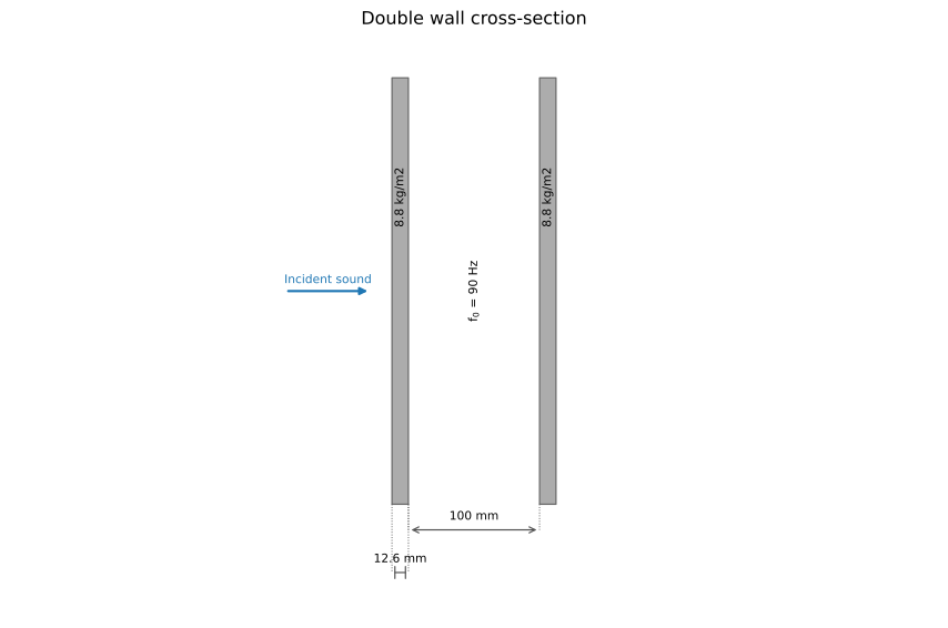
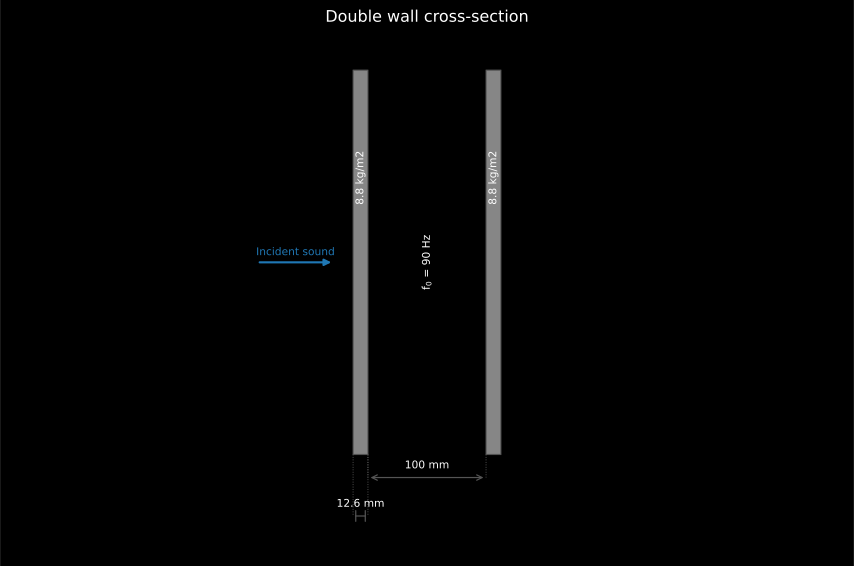
The whole model in one section: the two thin leaves are the masses, the 100 mm air gap is the spring, and $f_0$ = 90 Hz is where the dip of every double-wall curve sits.

Show the code for this figure

import matplotlib.pyplot as plt
from phonometry import mass_spring_mass_resonance, plot_double_wall_geometry

# Two 8.8 kg/m2 plasterboard leaves on a 100 mm cavity.
f0 = mass_spring_mass_resonance(8.8, 8.8, 0.1)
plot_double_wall_geometry(8.8, 8.8, 0.1, resonance_frequency=f0)
plt.show()

# A double-wall prediction retains its geometry and redraws it:
#   dw = double_wall_transmission_loss(bands, 8.8, 8.8, 0.1)
#   dw.plot_geometry()

Masonry cavity walls: the wall-tie bridge (Hopkins 4.3.5.4)

The double-wall model above treats the cavity as pure air. A real masonry cavity wall is stitched together by wall ties every few courses, and those ties do two things the air-only model cannot see: they add a mechanical spring in parallel with the air spring, which pushes the mass-spring-mass resonance up, and they open a structure-borne path from one leaf to the other.

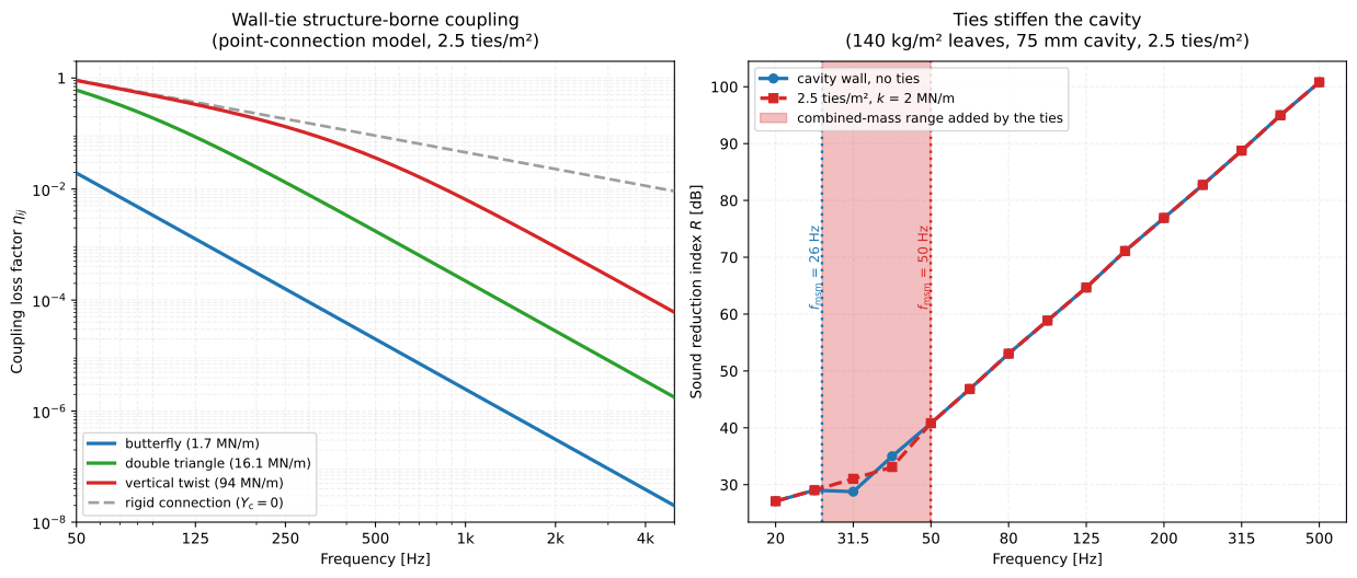
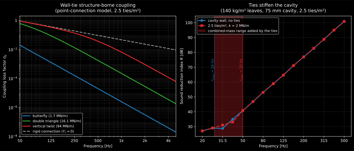
Left: a soft tie rolls the structure-borne coupling off as $1/f^3$, a stiff one stays on the rigid ceiling for another two octaves. Right: the same ties lift the resonance from 26 Hz to 50 Hz, extending the combined-mass branch. Both panels are built by the two snippets of this section: the right one by double_wall_transmission_loss with and without tie_stiffness_per_area, the left one by wall_tie_coupling_loss_factor(...).plot().

The tie as a spring (Hopkins Eq. 4.89). A tie is characterised by a single number, its dynamic stiffness $s_{X\text{mm}}$ at a cavity width $X$, measured on two nominally identical 100 mm concrete cubes (Section 3.11.3.2, Eq. 3.202). $N$ ties over a plate of area $S$ add $Nk/S$ to the cavity air stiffness:

$$f_{\text{msm}}=\frac{1}{2\pi }\sqrt{\frac{s_a+Nk/S}{{\rho }_{s1}{\rho }_{s2}/({\rho }_{s1}+{\rho }_{s2})}}.$$

Below $f_{\text{msm}}$ the two leaves act as one plate of the combined mass, so stiff ties are doubly bad: they raise the resonance into the rating range and bridge the cavity. WALL_TIE_STIFFNESS carries Hopkins’ Table A4, whose 50 mm rows come from Hopkins, Wilson & Craik (1999) and whose 100 mm row from Hall & Hopkins (2001).

Wall tie	Cavity width (mm)	$s_{X\text{mm}}$ (MN/m)
Butterfly tie (BS 1243:1978)	50	1.7
Double-triangle tie (BS 1243:1978)	50	16.1
Vertical-twist tie (BS 1243:1978)	50	94.0
Vertical-twist tie (proprietary)	100	43.4

from phonometry import (
    double_wall_transmission_loss,
    mass_spring_mass_resonance,
    wall_tie_stiffness,
    wall_tie_stiffness_per_area,
)

print(wall_tie_stiffness("butterfly"))        # (0.05 m, 1.7e6 N/m)

# Hopkins Fig. 4.35: two 140 kg/m2 leaves across an empty 75 mm cavity.
print(round(mass_spring_mass_resonance(140.0, 140.0, 0.075)))          # 26 Hz

# Add 2.5 ties per m2 of s_75mm = 2 MN/m: the resonance nearly doubles.
ties = wall_tie_stiffness_per_area(2.5, 2.0e6)
print(round(mass_spring_mass_resonance(140.0, 140.0, 0.075,
                                       tie_stiffness_per_area=ties)))  # 50 Hz

dw = double_wall_transmission_loss(bands, 140.0, 140.0, 0.075,
                                   tie_stiffness_per_area=ties)

The tie as a point connection (Hopkins Eqs. 4.84 to 4.88). Each tie transmits structure-borne power between the leaves. With the driving-point mobilities $Y_i$, $Y_j$ of the two leaves (infinite thin plates, $Y=1/(8\sqrt{B^{\prime }{m}^{\prime \prime }})$, Eq. 2.190) and the connector mobility of a linear spring $Y_c=\mathrm{i}\omega /k$ (Eq. 4.88), $N$ identical uncorrelated connections give the coupling loss factor (Eq. 4.87)

$${\eta }_{ij}=\frac{N}{\omega m_i}\frac{\mathrm{Re}\{Y_j\}}{|Y_i+Y_j+Y_c{|}^2}.$$

The plate area cancels ($N/m_i=n/{\rho }_{s1}$ with $n$ ties per m²), so only the tie density enters. A rigid connection (a screw, a nail, a bolt, or a tie stiff enough never to yield) is the limit $Y_c=0$; a resilient tie rolls the coupling off two powers faster once $|Y_c|=\omega /k$ overtakes the plate mobilities: ${\eta }_{ij}$ then falls as $1/f^3$ against the rigid ceiling’s $1/f$, so the ratio between them goes as $1/f^2$. That is exactly why a butterfly tie at 1.7 MN/m and a vertical-twist tie at 94 MN/m behave so differently.

import numpy as np
from phonometry import plate_bending_stiffness, wall_tie_coupling_loss_factor

freq = np.logspace(np.log10(50.0), np.log10(5000.0), 60)
b1 = plate_bending_stiffness(2.0e10, 0.1, 0.2)   # 100 mm masonry leaves
res = wall_tie_coupling_loss_factor(
    freq, 150.0, 170.0, b1, b1, ties_per_area=2.5, tie="butterfly"
)
print(res.coupling_loss_factor[0], res.rigid_coupling_loss_factor[0])
res.plot()   # eta_ij against the rigid-connection ceiling (needs matplotlib)

The inputs of this model are printed data: Table A4, confirmed value for value by Hopkins, Wilson & Craik (1999) Table 1, which prints the same 1.7 / 16.1 / 94.0 MN/m at a 50 mm cavity. Craik & Wilson (1995) Table 1 measures the same tie types at an 85 mm cavity and reports 1.1 and 4.3 MN/m for the butterfly and double-triangle ties, so it corroborates the ordering but not the values: the dynamic stiffness is defined at a given cavity width and changes with it. The output is not printed anywhere: every published sound reduction index of a bridged masonry cavity wall is a figure, so the per-band transmission-loss penalty of the ties has no printed numeric oracle. The resonance shift does: Hopkins Fig. 4.35 prints 26 Hz without ties and 50 Hz with them for the same wall.

Slits, holes and apertures (Hopkins 4.3.10)

A small air path is the real limit on any heavy construction. The transmission coefficient of a straight slit (Gomperts, Hopkins Eq. 4.99) and of a circular hole (Wilson & Soroka, Eq. 4.102) are predicted directly, with the slit’s resonances at $d+2e=z\lambda /2$ (Eq. 4.101). They combine with the wall in the area-weighted energy sum (Eq. 4.92)

$$R=-10{\log }_{10}\left(\frac{1}{{\sum }_n{S}_n}\sum _n{S}_{n}10^{-R_n/10}\right),$$

so a bare opening of relative area $S_a/S$ caps the composite at $10{\log }_{10}(S/S_a)$; a 1 % opening can never do better than 20 dB, whatever the wall.

from phonometry import (
    composite_transmission_loss, slit_transmission_coefficient,
    slit_resonance_frequencies,
)

# A 2 mm x 100 mm-deep slit: its transmission peaks at the half-wavelength
# resonances of the slit depth.
print(slit_resonance_frequencies(depth=0.1, width=0.002, orders=2).round().tolist())  # [~1500, ~3100]

# A wall of Rw = 50 dB with 1 % of its area left open as a slit is capped:
print(round(float(composite_transmission_loss([0.99, 0.01], [50.0, 0.0])), 1))   # 20.0

The leak that undoes a heavy wall is almost invisible, and .plot_geometry() makes the point by drawing it to scale: a 2 mm gap through 100 mm of masonry.

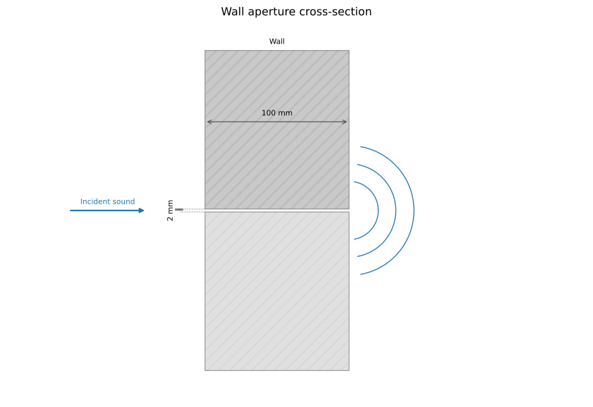
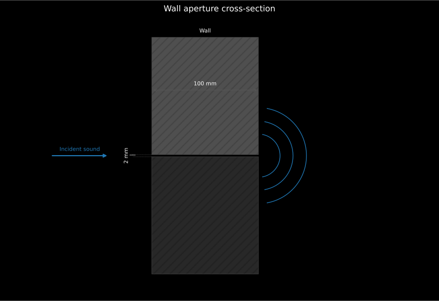
The tiny geometry behind a large leak: the gap is 50 times deeper than it is wide, which is why it behaves as a short tube with half-wavelength depth resonances near 1.5 and 3.1 kHz rather than as a simple open area.

Show the code for this figure

import matplotlib.pyplot as plt
import numpy as np
from phonometry import slit_transmission_coefficient

f = np.geomspace(100.0, 5000.0, 200)
result = slit_transmission_coefficient(f, width=0.002, depth=0.1)

# One line: the wall section with the slit to scale.
result.plot_geometry()
plt.show()

The clip below puts the two regimes side by side in a 2D FDTD field: a plane front meets a rigid 0.10 m wall with a 25 mm slit (λ/20 at 686 Hz) and with a 0.50 m opening (one wavelength). The narrow slit re-radiates what it swallows as a cylindrical wave, the Gomperts transmission of the model annotated; the wavelength-sized opening lets the front through nearly intact and casts sharp-edged shadows. What the slit passes is about 23 dB under the standing wave that faces the wall, so in the instantaneous panels the half space behind the wall rides the display gain each panel prints (x10, that is +20 dB, for the slit and none for the wavelength-sized opening); the RMS maps below keep one shared scale, which is where the two openings are compared level for level.

A 686 Hz plane wave in a 2D FDTD field hits a rigid wall with a 25 mm slit and, in a second panel, a 0.50 m opening. The narrow slit re-radiates a cylindrical wave into the half space behind, drawn with an annotated ten-fold display gain (+20 dB) and with the Gomperts transmission coefficient of 0.55 annotated; the wavelength-sized opening passes a beam with sharp-edged shadows at unit gain, both RMS maps on the same colour scale.

Download the animation (WebM)

A 686 Hz plane wave in a 2D FDTD field hits a rigid wall with a 25 mm slit and, in a second panel, a 0.50 m opening. The narrow slit re-radiates a cylindrical wave into the half space behind, drawn with an annotated ten-fold display gain (+20 dB) and with the Gomperts transmission coefficient of 0.55 annotated; the wavelength-sized opening passes a beam with sharp-edged shadows at unit gain, both RMS maps on the same colour scale.

Download the animation (WebM)

Radiation efficiency of a bending plate (Hopkins 2.9)

How much airborne power a vibrating plate actually radiates per unit mean-square velocity is its radiation efficiency $\sigma$, the radiation factor $\epsilon$ that Sound Power from Surface Vibration (ISO 7849) otherwise takes as a measured input. It is defined as the ratio of the power the plate actually radiates to the power a rigid piston of the same area and the same mean-square velocity would radiate, so $\sigma =1$ means “as efficient as a piston” — and, as the numbers below show, a plate can beat that near coincidence.

There are three regimes, not two (Leppington/Maidanik, Hopkins Eqs 2.227-2.230). Well below $f_c$ the bending wavelength is shorter than the acoustic one, adjacent half-waves cancel each other’s volume flow, and only the uncancelled strips at the edges and corners radiate. That is why the calculation needs the plate’s two dimensions and its edge condition: a clamped edge radiates more than a simply supported one, and a plate with baffles perpendicular to its edges more than one flush in an infinite baffle — the boundary and baffle arguments select between them. Around $f_c$ the trace wavelength of the bending wave matches the acoustic wavelength, the Leppington form $(1-f_c/f{)}^{-1/2}$ diverges and is capped by the at-coincidence expression; the pane below peaks at $\sigma =2.6$ in the 2 kHz band. Only far above $f_c$ does $\sigma$ settle towards 1: a third of an octave past coincidence this pane is still at 1.74.

$$\sigma =\frac{1}{\sqrt{1-f_c/f}}(f>f_c),\sigma \to 1(f\gg f_c).$$

Two consequences are worth carrying away. A small plate is a relatively better radiator than a large one of the same material below $f_c$, because the radiating edge strip is a larger fraction of it: the 1.5 × 1.25 m pane below gives $\sigma =0.011$ at 100 Hz, a 0.5 × 0.4 m pane of the same glass 0.034. And the coincidence dip in $R$ and the coincidence peak in $\sigma$ are the same event seen from the two sides — the same $\sigma$ reappears in the transmission factor of the detailed EN 12354 model and as the radiation factor ISO 7849 measures.

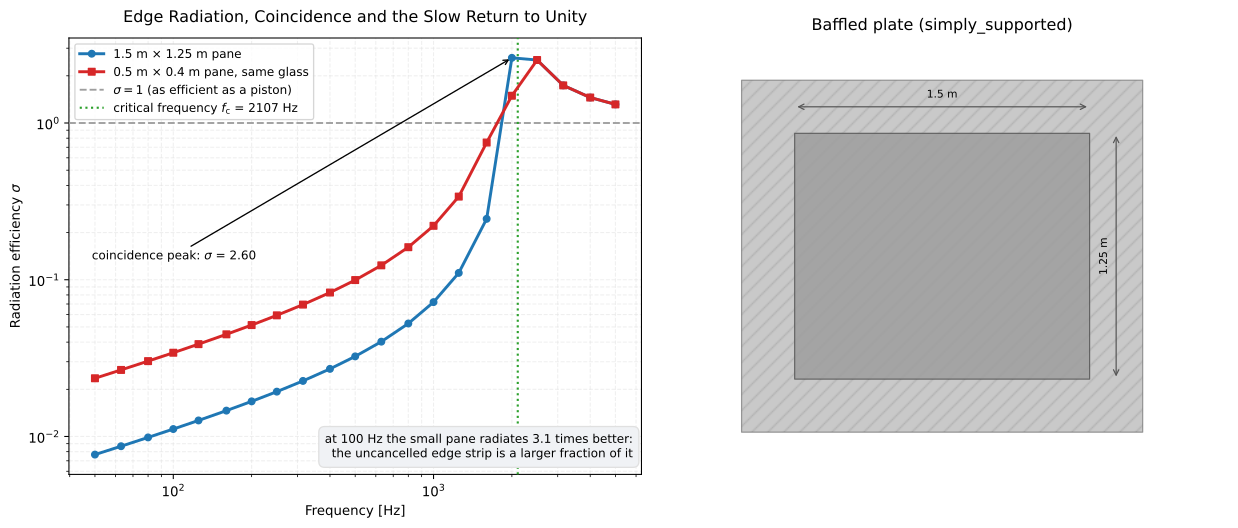
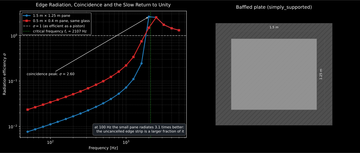
Three regimes on one axis. Below $f_c$ the two panes differ by a factor of three in $\sigma$ although they are the same glass — the smaller one radiates relatively better, because its uncancelled edge strip is a larger fraction of it. At coincidence both peak above unity, the 1.5 × 1.25 m pane at 2.61 in the 2 kHz band that straddles $f_c$ = 2 107 Hz. Above it $\sigma$ falls back towards 1 only slowly: still 1.74 one third of an octave past coincidence and 1.32 at 5 kHz. The right-hand panel is the geometry the model assumes and the reason it needs two dimensions and an edge condition.

Show the code for this figure

import matplotlib.pyplot as plt

sig_big = radiation_efficiency(bands, 1.5, 1.25, fc)
sig_small = radiation_efficiency(bands, 0.5, 0.4, fc)

fig, (ax_l, ax_r) = plt.subplots(1, 2, figsize=(11, 4.5))
ax_l.loglog(bands, sig_big.radiation_efficiency, "-o", ms=3, label="1.5 x 1.25 m")
ax_l.loglog(bands, sig_small.radiation_efficiency, "-s", ms=3, label="0.5 x 0.4 m")
ax_l.axhline(1.0, ls=":")
ax_l.axvline(fc, ls=":", color="r")
ax_l.set(xlabel="Frequency [Hz]", ylabel=r"Radiation efficiency $\sigma$")
ax_l.legend()

# One line — the baffled plate the model assumes:
sig_big.plot_geometry(ax=ax_r)
plt.show()

from phonometry import radiation_efficiency, sound_power_from_vibration

# The 6 mm glass pane (1.5 x 1.25 m) of the single-panel example above.
sig = radiation_efficiency(bands, 1.5, 1.25, fc)
print(sig.radiation_efficiency[bands == 2000].round(2))
# 2.6, the coincidence peak: the plate out-radiates a piston near fc

# Feed the prediction straight into ISO 7849 as the radiation factor:
lw = sound_power_from_vibration(velocity_level=80.0, area=1.875,
                                radiation_factor=sig.radiation_efficiency,
                                frequencies=bands)

sig.plot()   # sigma(f) with the coincidence peak (needs matplotlib)

Point mobilities of infinite structures (Cremer Table 5.1)

The vibrational power a point force injects is $W=\frac{1}{2}|F{|}^2\mathrm{Re}\{Y\}$ (Cremer Eq. 5.23), so the driving-point mobility $Y$ (the reciprocal of the impedance) sets how much energy a structure absorbs. For infinite structures these are closed forms: an infinite thin plate is a pure resistance $Z=8\sqrt{B^{\prime }{m}^{\prime \prime }}$ (real, frequency independent), while an infinite beam has $Y=(1-\mathrm{j})/(4m^{\prime }{c}_B)$ (45 degrees, falling as ${\omega }^{-1/2}$). They supply the receiver mobility EN 12354-5 needs when no measurement exists. infinite_plate_point_mobility and infinite_beam_point_mobility return the same quantities bundled as an ISO 7626 MobilityResult, so they plot, convert and report like any measured FRF; the mechanical mobility guide reads them against the SDOF resonator and adds the moment and longitudinal-rod cases.

from phonometry import infinite_plate_impedance, infinite_beam_mobility, injected_power

z_plate = infinite_plate_impedance(bp, mass)          # Z = 8 sqrt(B' m'') [N.s/m]
print(round(z_plate))                                 # real, frequency independent
w = injected_power(force=10.0, mobility=1.0 / z_plate)
print(round(float(w) * 1e3, 3), "mW")                 # W = |F|^2 / (16 sqrt(B' m''))

Function parameters

Parameter	Type	Units	Range / default	Notes
mass_per_area	float	kg/m²	> 0	Surface density $m^{\prime \prime }$
critical_frequency / bending_stiffness	float	Hz / N·m	give one	Coincidence $f_c$, or $B^{\prime }$ to compute it
loss_factor	float	—	> 0; default 0.01 single panel, 0.1 double wall	Total loss factor $\eta$
band	str	—	'third' (−5.5 dB) / 'octave' (−4.0 dB)	Field-incidence correction width
mass1 / mass2	float	kg/m²	> 0	Double-wall leaf surface densities
gap	float	m	> 0	Cavity depth $d$
cavity_medium	PorousMediumResult	—	default None	Porous fill; lowers $f_0$
width (slit)	float	m	> 0	Slit width $w$. Second positional argument of both slit_transmission_coefficient and slit_resonance_frequencies
depth (slit)	float	m	> 0	Slit depth $d$ (the wall thickness). Third positional argument of slit_transmission_coefficient, first of slit_resonance_frequencies — the two functions take the pair in opposite orders
field / position (slit)	str	—	'diffuse'/'normal', 'mid'/'edge'	Incident field and slit location
radius / depth (hole)	float	m	> 0	Circular-aperture radius $a$ / depth $d$
areas / reduction_indices	seq	m² / dB	length $N$	Composite elements (1-D or (N, bands))
length_x / length_y	float	m	> 0	Plate dimensions (radiation efficiency)
boundary / baffle	str	—	'simply_supported'/'clamped', 'infinite'/'perpendicular'	Plate edge and baffle constants

single_panel_transmission_loss and double_wall_transmission_loss return a SoundReductionResult (transmission_loss, transmission_coefficient, critical_frequency / resonance_frequency, .rating(), .plot()); the slit and hole functions return an ApertureTransmissionResult (transmission_coefficient, transmission_loss, .plot()); radiation_efficiency a RadiationEfficiencyResult (radiation_efficiency, radiation_index, .plot()). The predictions carry the modelling caveats of their sources (Sharp’s method above $1.5\times$ the first panel resonance; Gomperts’ inviscid slit valid for $w<0.3\lambda$; Leppington “method no. 1”).

What this guide covers

• Covered

  The source formulae themselves: Bies’ §7.2 mass law and Sharp’s coincidence method (Eqs 7.40/7.42/7.44) for a single panel, the double-wall mass-spring-mass resonance and its saturating cavity boost (Eqs 7.62-7.64), Hopkins’ Gomperts slit and Wilson & Soroka circular-hole transmission coefficients with the area-weighted composite sum (Eq. 4.92), the Leppington/Maidanik plate radiation efficiency (Eqs 2.227-2.230), and the Cremer Table 5.1 point impedances and mobilities of infinite plates and beams with the injected-power relation, via single_panel_transmission_loss, double_wall_transmission_loss, slit_transmission_coefficient, composite_transmission_loss, radiation_efficiency, infinite_plate_impedance, infinite_beam_mobility and injected_power. Vigran’s orthotropic chapter joins them: the coincidence range of a ribbed or corrugated panel and its flattened transmission loss by either the diffuse-field integral or Heckl’s closed form (Eqs 6.107-6.113), the Timoshenko equivalent stiffnesses of a sinusoidal corrugation (Eq. 3.115) and the orthotropic plate eigenfrequency (Eq. 3.113), via orthotropic_transmission_loss, orthotropic_critical_frequencies, corrugated_plate_stiffness, corrugated_plate_mass_factor and orthotropic_plate_resonance. Masonry cavity walls add the wall-tie bridge of Hopkins’ Sections 3.11.3.2 and 4.3.5.4.1: the Table A4 dynamic stiffnesses, the tie array acting in parallel with the cavity air (Eq. 4.89, reached through the tie_stiffness_per_area keyword of mass_spring_mass_resonance and double_wall_transmission_loss) and the point-connection coupling loss factor with a linear-spring connector (Eqs 4.87 and 4.88), via wall_tie_stiffness, wall_tie_stiffness_per_area and wall_tie_coupling_loss_factor.

• Not covered

  Each prediction stays inside the validity range its source states, which the guide flags but does not extend past: Sharp’s method (and so single_panel_transmission_loss) is not valid below about $1.5\times$ the panel’s first resonance, where the panel’s own low-frequency modal behaviour, not the mass law, governs; Gomperts’ slit model holds only for a narrow slit, $w<0.3\lambda$, so a wide aperture falls outside it; and only Leppington’s “method no. 1” for radiation efficiency is implemented, not his other published formulations. The orthotropic models are infinite-panel models on the same footing: below about $0.7f_{c1}$ Heckl’s branch underestimates $R$ on small panels, and the 2 kHz to 4 kHz dip that real corrugated cladding shows comes from resonances of the panel sections between the ribs, which neither route predicts. Only the sinusoidal (“wavy”) corrugation has equivalent stiffnesses here; trapezoidal cladding needs its own, from the literature Vigran cites. The wall-tie model is on the same footing on its output side: the inputs are printed data, but no published sound reduction index of a bridged masonry cavity wall is tabulated, so the per-band penalty the ties cause has no numeric oracle and only the resonance shift is anchored (Hopkins Fig. 4.35, 26 Hz to 50 Hz). The coupling loss factor is not fed into a full statistical energy analysis here; combining it with the airborne path would need the whole room-plate-cavity-plate-room chain.

See also

• Predicting Sound Insulation (EN 12354): assembles predicted or measured element $R$ into the in-situ $R_w^{\prime }$.
• Sound Power from Surface Vibration (ISO 7849): consumes the predicted radiation efficiency as its radiation factor.
• Mechanical mobility and the FRF family (ISO 7626-1): the measured counterpart of the theoretical point mobilities.
• Porous and multilayer absorbers: the cavity-fill models a double wall consumes.
• API reference: building.prediction.panel_transmission, building.prediction.masonry_cavity_wall, building.prediction.aperture_transmission, vibration.structural.radiation_efficiency and vibration.structural.point_mobility.
• Theory: Sound insulation and absorption, predicted: the mass law, the coincidence dip and the transmission coefficient the panel models return.

References

• Bies, D. A., Hansen, C. H., & Howard, C. Q. (2017). Engineering Noise Control (5th ed.). CRC Press. https://doi.org/10.1201/9781351228152Section 7.2: the mass law (Eq. 7.40/7.42), coincidence frequency (Eq. 7.3), Sharp's single-panel method (7.2.4.1) and the double-wall model (7.2.6, Eq. 7.62-7.64). ISBN 978-1-4987-2405-0.
• Craik, R. J. M., & Wilson, R. (1995). Sound transmission through masonry cavity walls. Journal of Sound and Vibration 179(1), 79-96. https://doi.org/10.1006/jsvi.1995.0006Table 1: the same tie types measured at an 85 mm cavity (butterfly 1,1 MN/m, double-triangle 4,3 MN/m), which corroborate the ordering of Table A4 but not its values, since the dynamic stiffness is defined at a given cavity width.
• Cremer, L., Heckl, M., & Petersson, B. A. T. (2005). Structure-Borne Sound (3rd ed.). Springer. https://doi.org/10.1007/b137728Chapter 5, Table 5.1: the compilation of point impedances and mobilities of infinite structures (plate Z = 8 sqrt(B' m''), beam, rod) and the injected-power relation W = 0.5 |F|^2 Re{Y} (Eq. 5.23). ISBN 978-3-540-22696-3.
• Hall, R., & Hopkins, C. (2001). The measurement of dynamic stiffness of wall ties used in masonry cavity walls. Proceedings of the Institute of Acoustics 23(8), 259-266. The 100 mm cavity row of Hopkins' Table A4: the proprietary vertical-twist tie at 43,4 MN/m.
• Hopkins, C. (2007). Sound insulation. Butterworth-Heinemann. https://doi.org/10.4324/9780080550473Section 2.9 (plate radiation efficiency, Leppington/Maidanik Eqs 2.227-2.230) and Section 4.3.10 (slits, holes and apertures, Gomperts Eq. 4.99, Wilson & Soroka Eq. 4.102, composite Eq. 4.92). ISBN 978-0-7506-6526-1.
• Hopkins, C., Wilson, R., & Craik, R. J. M. (1999). Dynamic stiffness as an acoustic specification parameter for wall ties used in masonry cavity walls. Applied Acoustics 58, 51-68. https://doi.org/10.1016/S0003-682X(98)00068-1The measurement behind the 50 mm rows of Hopkins' Table A4: butterfly 1,7 MN/m, double-triangle 16,1 MN/m and vertical-twist 94,0 MN/m.
• Norton, M. P., & Karczub, D. G. (2003). Fundamentals of noise and vibration analysis for engineers (2nd ed.). Cambridge University Press. https://doi.org/10.1017/CBO9781139163927Section 3.9.1: the plateau method after Watters, with Table 3.1 (surface density per millimetre, plateau height and the B/A frequency ratio) behind PLATEAU_MATERIALS; Eqs. 3.104/3.106 (field-incidence mass law), Eq. 3.110 (the above-coincidence branch of the coincidence_model='cremer' variant) and problem 3.11, the worked brick wall reproduced here. ISBN 978-0-521-49913-2.
• Vigran, T. E. (2008). Building Acoustics. Taylor & Francis. https://doi.org/10.1201/9781482266016Sections 3.7.3.3 (orthotropic plate eigenfrequencies, Eqs 3.113-3.115 after Timoshenko & Woinowsky-Krieger) and 6.5.3 (orthotropic panel transmission, Eqs 6.107-6.113 after Heckl 1960 and Hansen 1993). ISBN 978-0-415-42853-8.