Elastic waves and fluid-solid coupling

Key references: Virieux 1986 Moczo et al. 2007 Cremer et al. 2005 Brekhovskikh & Godin 1990 van Vossen et al. 2002

A fluid carries one wave; a solid carries a family of them. This guide covers the elastic companion of the 2D FDTD wave simulation: elastic_fdtd_simulation integrates the plane-strain velocity-stress system of Virieux (1986) on the same staggered grid as the acoustic solver, and with it the compressional P wave, the shear S wave, the Rayleigh wave of a free surface and the Scholte wave of a fluid-solid contact all emerge from the same update. Because a fluid is just the shear-free limit of the elastic equations, one pair of material maps couples water, air, sediment and steel in a single run: oblique reflection with mode conversion, seabed interface waves and the transmission of immersed plates come out of the maps alone, each pinned to its exact closed form by the validation suite.

The guide assumes the acoustic solver’s vocabulary (sources, probes, obstacle masks, sponges and the Courant bound); read 2D FDTD wave simulation first if those are new. The closed forms this solver cross-checks live in the building, vibration and underwater guides: the mass law of panel sound insulation, the flexural waves of bending-wave transmission at plate junctions, and the shear-supporting seabed that the fluid-bottom reflection model of underwater sound propagation cannot represent.

1. The P-SV velocity-stress scheme

A solid carries more than one wave. Alongside the compressional P wave at $c_{P} = (λ + 2 μ) / ρ$ a shear S wave propagates at $c_{S} = μ / ρ$ , and every traction-free surface guides a Rayleigh wave just below $c_{S}$ . elastic_fdtd_simulation integrates the 2D plane-strain velocity-stress system of Virieux (1986, Eq. 2),

ρ \frac{\partial v}{\partial t} = \nabla \cdot τ, \frac{\partial τ}{\partial t} = λ (\nabla \cdot v) I + μ (\nabla v + \nabla v^{T}),

on the same staggered layout as the acoustic solver: the normal stresses txx/tyy share the cell centres where the acoustic pressure lives, the velocities sit on the faces and the shear stress txy on the corners (Virieux’s fully staggered cell, shifted half a cell). The API mirrors fdtd_simulation piece by piece: wave-speed maps c_p and c_s (plus rho) instead of c, ExplosionSource (an isotropic stress injection) and ForceSource (a directional body force) as sources, probes that record p, vx or vy, the same sponge and obstacle machinery, and a frozen ElasticFDTDResult with the same .plot(). What the run writes down travels as one ElasticRecording (the probe cells and their fields, the snapshot cadence and its field) and how the domain ends as one ElasticBoundaries (the sides and the sponge thickness).

Two numbers govern every run, and they read opposite ends of the material maps. Stability: the time step follows the fastest wave in the domain, $c_{P}^{m a x}$ , exactly as in the acoustic solver (Virieux Eqs. 6-7). Resolution: the cell size follows the slowest, $Δ x \leq c_{min} / (10 f)$ , where $c_{min}$ is the slowest non-zero shear speed among the solid cells — or a fluid $P$ speed, if some fluid region is slower still. In a wholly solid map the shear wavelength is always the shortest; in a mixed map it need not be, as with water at 1480 m/s over a sediment whose shear speed is 2000 m/s.

Those two ends are what a high-contrast domain costs. Δx is fixed by the slowest medium and Δt by the fastest, so the number of steps needed to cover a given physical time grows with the ratio of the two speeds: a water-over-steel domain resolved for the water wavelength still has to step at the steel’s 5900 m/s, roughly four times more steps than the same domain filled with water alone. The slow regions then run at a much lower local Courant number, where the dispersion error of the scheme is nearest its worst-case bound, so their effective resolution is poorer than the cell count suggests — which is why the ten-cell rule is a floor rather than a target in high-contrast problems. When only one medium carries the physics of interest, replacing the other by a boundary condition — an impedance edge or a sponge — is usually far cheaper than meshing both.

import numpy as np
from phonometry import simulation

# An aluminium block hit by a tiny explosion: the P front reaches two
# probes 100 and 220 cells away; c_P falls out of the differential delay.
w = 8e-6
res = simulation.elastic_fdtd_simulation(
    6320.0, 3130.0, 0.002, 1.1e-4, rho=2700.0, shape=(501, 501),
    sources=[simulation.ExplosionSource(
        ix=250, iy=250,
        waveform=simulation.GaussianPulse(0, 0, width=w).value)],
    recording=simulation.ElasticRecording(
        probes=[(350, 250), (470, 250)], probe_fields=("p",)),
)
t = res.times[1:]
t1, t2 = (t[np.abs(res.signals[k, 0, 1:]).argmax()] for k in range(2))
print(round(0.24 / (t2 - t1)))    # 6316  c_P = sqrt((lambda+2mu)/rho) = 6320

2. Fluids inside the elastic solver

Setting c_s = 0 marks a fluid cell: the shear modulus vanishes, the system degenerates to the acoustic equations, and with a uniform c_s = 0 map the elastic solver reproduces the acoustic one bit for bit (the regression suite asserts exact equality). That equivalence is a correctness guarantee, not a recommendation: this solver carries three stress fields where the acoustic one carries a single pressure, so an all-fluid problem costs roughly twice the memory and stepping time here. Use the acoustic solver unless some part of the domain supports shear.

A water column over a steel half-space is therefore just two bands of the material maps: with the density averaged arithmetically onto the faces and the shear modulus harmonically onto the corners (Moczo et al. 2007, Eqs. 7.37-7.39), the traction continuity of every internal interface, fluid-solid contacts included, emerges from the maps alone. The validation suite measures the normal-incidence reflection of a water-steel interface within 2 % of $(Z_{2} - Z_{1}) / (Z_{2} + Z_{1})$ (typically a fraction of a percent) and recovers the normal-incidence mass law of a 3 mm immersed steel plate within 0.3 dB of mass_law_transmission_loss.

Where the contact actually sits, and how to check it. A region painted from row $i$ downward puts the physical interface on the face plane at $y = i Δ x$ , because that is where the density is averaged onto the faces and the shear modulus onto the corners. Distances quoted “from the contact” should be measured from that plane, and a probe belongs several cells clear of it so it never samples the averaged cells. Verify a painted map before running it — plt.imshow(sim.c_s) with the region borders drawn on, or simply asserting the row index of the first solid row — because a one-row error moves every arrival by $Δ x / c$ and costs a whole run. There is no elastic counterpart of FDTD2D.plot_geometry, so this check is the reader’s own. One more failure is worth knowing in advance: every cell must satisfy $c_{P}^{2} \geq 2 c_{S}^{2}$ , which the constructor enforces, and that rejection is the first thing to look at when a sediment or composite map will not build.

3. Free surfaces and Rayleigh waves

Every side is rigid unless you declare otherwise, and rigid here means clamped. The boundary holds the particle velocity at zero, so it reflects with the opposite polarity of a free surface and supports no surface wave at all. That is the right model for a body continuing into something much stiffer, and the wrong one for a body in air or in vacuum — which is what most structural problems are. A plate, block or beam meant to be free must therefore have every exposed side declared free, and the symptom of forgetting is quiet: the wavefronts still look plausible, but the Rayleigh train the figure below makes obvious is simply missing, the reflections come back inverted, and no free-plate closed form matches. The third option is "absorbing", which terminates a half-space so the domain edge is not seen at all; the three are chosen per side, which is exactly how the half-space example works — free on top, absorbing on the other three. Since there is no elastic counterpart of FDTD2D.plot_geometry, read the boundary spec back off the ElasticBoundaries object before committing to a long run.

A side declared "free" becomes a traction-free surface through stress imaging (Moczo et al. Eq. 9.9): the normal stress is pinned to zero on the surface plane and the shear stress above it is its antisymmetric image. That single boundary condition is what makes surfaces wave-bearing: strike the free surface of an aluminium block vertically (Lamb’s problem) and, besides the P and S body fronts, a Rayleigh wave rolls along the surface at $c_{R} \approx 0.93 c_{S}$ , the root of the exact Rayleigh characteristic equation (Cremer, Heckl & Petersson Eq. 3.149). The tests pin the measured Rayleigh speed to that root within 2 % and the flexural wave of a thin free-free strip to the Kirchhoff plate dispersion $c_{B} \propto ω$ in its thin-plate domain. Free surfaces ride the Rayleigh sampling rule: allow 15-20 cells per wavelength there, the second-order imaging surface being the most dispersive part of the scheme.

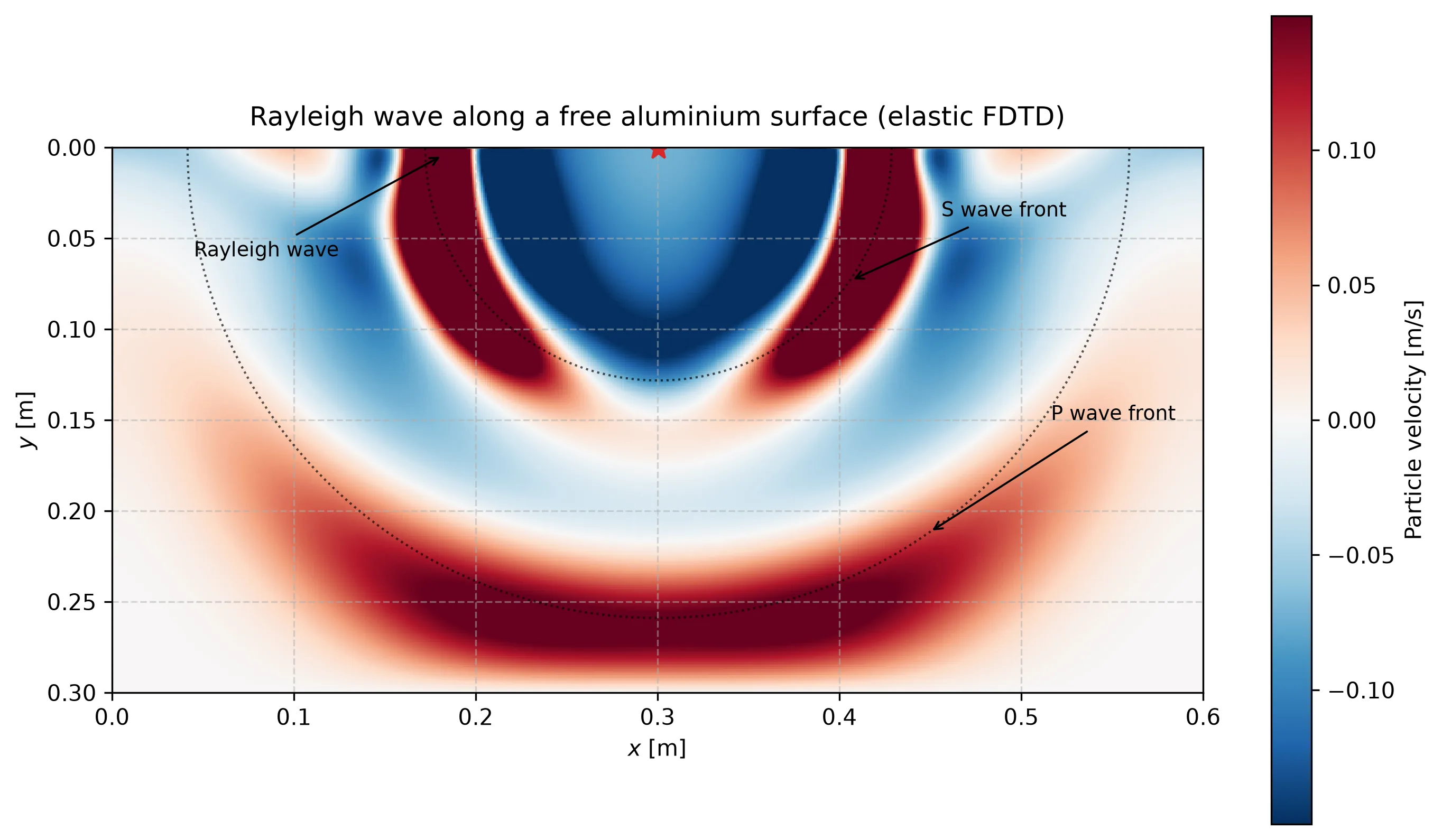
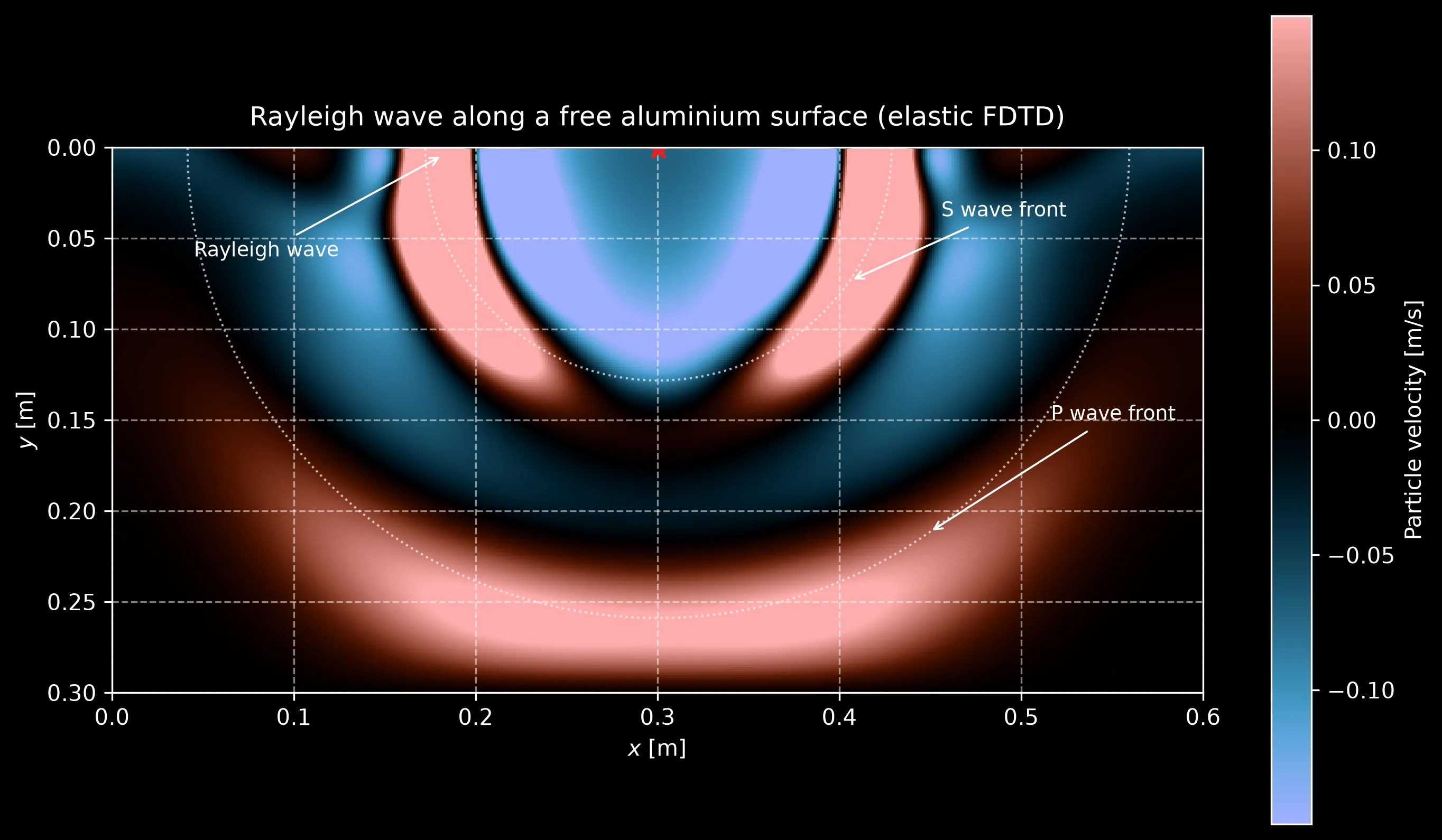
Snapshot of the vertical particle velocity in a 0.6 by 0.3 metre aluminium block a few hundredths of a millisecond after a vertical hit on its free upper surface: the compressional P front is the outer arc, the shear S front the inner arc at about half its radius, and the strongest lobes hug the surface just behind the S front, labelled as the Rayleigh wave; dotted arcs mark the exact P and S radii

One snapshot, three speeds: the P front has covered twice the distance of the S front (dotted arcs at the exact $c_{P} t$ and $c_{S} t$ radii), and the strongest motion travels along the free surface as the Rayleigh wave, a whisker slower than S.

A sponge is the wrong tool where this page’s physics lives. There is no elastic perfectly matched layer here, and the sponge absorbs a grazing Rayleigh or Scholte wave far less effectively than a body wave, precisely because a surface-guided wave runs along the layer instead of into it. Three consequences worth acting on. A side cannot be both free and absorbing, so where a free surface meets a sponge at a corner the imaged stresses and the absorption ramp work against each other: keep the source at least a wavelength from that corner and end the run before the surface wave reaches it. An interface or surface wave needs a thicker layer than a body wave — start at roughly twice the width you would use for P and S, then verify by extending the run and watching for a return. And when only the early arrivals matter, plain rigid sides with a run shorter than the first wall echo are cleaner than any sponge: that is exactly what the snapshot above does, at 73 µs on a 0.6 m block whose nearest side-wall P return arrives at 95 µs and whose Rayleigh wave reaches the corner at 103 µs.

Show the code for this figure

import numpy as np
import matplotlib.pyplot as plt
from phonometry import simulation

# A 0.6 x 0.3 m aluminium block, struck vertically at its free surface.
dx, w = 0.001, 8e-6
dt = 0.6 * dx / (6320.0 * np.sqrt(2.0))
steps = round(7.3e-5 / dt)
res = simulation.elastic_fdtd_simulation(
    6320.0, 3130.0, dx, 7.3e-5, rho=2700.0, shape=(300, 600),
    sources=[simulation.ForceSource(
        ix=300, iy=0, direction="y", amplitude=1e6,
        waveform=simulation.GaussianPulse(0, 0, width=w).value)],
    boundaries=simulation.ElasticBoundaries({"top": "free"}),
    recording=simulation.ElasticRecording(snapshot_every=steps,
                                          snapshot_field="vy"),
)
res.plot(kind="snapshot")
plt.show()

The snapshot stops at 73 µs because rigid sides and a short run were the cheapest way to get one clean frame, and one frame is enough for the two body speeds: the dotted arcs are drawn at the exact $c_{P} t$ and $c_{S} t$ radii, so they are a measurement and not a label. What one frame cannot settle is the third wave. Nothing analytic is drawn for it, its speed differs from the shear front’s by 7 %, and its defining property — it stays on the surface while the body fronts leave — is a statement about what happens next.

So run the same hit for 163 µs instead, with sponges on the other three sides and the domain widened until the corner where a sponge meets the free surface is outside the frame, and run it twice: once with the top declared "free" and once with it left at the solver default, the clamped rigid wall. Same aluminium, same hit, same two body fronts — and no surface train at all in the second. That is the claim of this section, drawn: the boundary condition makes the Rayleigh wave, not the material.

Download the animation (WebM)

Watch what the fronts do at the end. Both body arcs run out of the frame and keep going; the surface lobes do not go anywhere but along the surface, at their own slower speed, and they are still there when the body waves have left. The inset traces two surface probes 0.15 m apart, and the delay between their peaks is the measurement: the simulated $c_{R}$ against 2921 m/s, the root of the exact Rayleigh characteristic equation quoted above, which the tests pin to within 2 %.

The two field panels are drawn on their own colour scales, and the clip says so, because a vertical force applied on a clamped surface nearly cancels against its own image and that run radiates far less than the free one. The probe traces below them keep a single shared scale, which is where the comparison stays quantitative: the missing surface arrival is a missing peak, not a rescaled one.

The other wave a free surface makes possible — the flexural wave of a thin free-free strip, the one pinned to the Kirchhoff dispersion above — is worth watching in motion too. The clip below is this same solver launching a 4 kHz bending packet along a 10 mm steel plate: on the control panel the plate runs straight and the packet simply leaves, and on the junction panel a perpendicular plate of the same thickness turns the corner into a scatterer. The packet splits there into the reflected and transmitted bending waves the closed form prices at $τ_{12} (0°) = 0.5$ , plus the fast in-plane precursor that races ahead down the receiving plate — the mode conversion the pinned-junction model deliberately leaves out, and the reason this page needs an elastic solver rather than a flexural one. The bending-wave transmission guide takes the same run apart against the EN 12354 vibration reduction index.

Download the animation (WebM)

4. Fluid-solid coupling at normal incidence

Because the fluid is just the c_s = 0 limit of the elastic scheme, a water-steel contact is one solver, two bands of the material maps, and the whole physics of fluid-solid coupling comes out of the same update. The Material constants and ElasticFDTD2D.from_regions build those layered maps without manual array surgery: a background material and a list of painted regions.

A Material is three measurable numbers — the compressional speed, the shear speed and the density — and a zero shear speed marks a fluid. Five constants ship, and every number elsewhere on this page comes out of them:

Constant	$c_{P}$ [m/s]	$c_{S}$ [m/s]	$ρ$ [kg/m³]
`AIR`	343	0	1.2
`WATER`	1480	0	1000
`CONCRETE`	3800	2250	2400
`STEEL`	5900	3200	7850
`ALUMINIUM`	6320	3130	2700

They are nominal round figures for documentation and validation, not certified data, so a real specimen should be entered by hand — which is why section 1 writes the aluminium block’s 6320 / 3130 / 2700 out rather than importing ALUMINIUM. The constructor enforces one bound, $c_{P}^{2} \geq 2 c_{S}^{2}$ : that is the statement that the first Lamé parameter is non-negative, equivalently that Poisson’s ratio is not negative. A rejected triple usually means a shear speed entered too high, or a compressional speed measured on a thin bar rather than in bulk — the thin-bar speed is the lower of the two, and substituting one for the other is a common error.

import numpy as np
from phonometry.simulation import ElasticFDTD2D, STEEL, WATER

# A 12 m water column over a steel half-space, as a 1D-like strip.
dx = 0.005
sim = ElasticFDTD2D.from_regions(
    (2400, 3), dx, background=WATER, regions=[(np.s_[1200:, :], STEEL)])
y = (np.arange(2400) + 0.5) * dx
p0 = np.exp(-(((y - 3.0) / 0.15) ** 2))[:, None]     # plane pulse
sim.txx[:] = -p0
sim.tyy[:] = -p0
y_face = np.arange(1, 2400) * dx + 0.5 * WATER.c_p * sim.dt
sim.vy += (np.exp(-(((y_face - 3.0) / 0.15) ** 2))
           / (WATER.rho * WATER.c_p))[:, None]       # one-way, leapfrog-consistent
trace = []
for _ in range(round(3.4e-3 / sim.dt)):
    sim.step()
    trace.append(sim.p[900, 1])
trace = np.asarray(trace)
t = (np.arange(trace.size) + 1) * sim.dt
incident = trace[t < 1.8e-3].max()
echo = trace[t > 2.6e-3]
print(round(float(echo[np.abs(echo).argmax()] / incident), 3))   # 0.938
# (Z2 - Z1)/(Z2 + Z1) = 0.938: at normal incidence no shear is excited
# and the steel behaves as a liquid of its rho and c_P (B&G Eq. 4.2.27)

That 0.938 is a ratio between two events on one trace, and the trace is where you see whether the run was clean enough to quote it. ElasticFDTDResult.plot() draws exactly this by default — probe histories, not field maps; the snapshots of sections 3 and 6 are .plot(kind="snapshot").

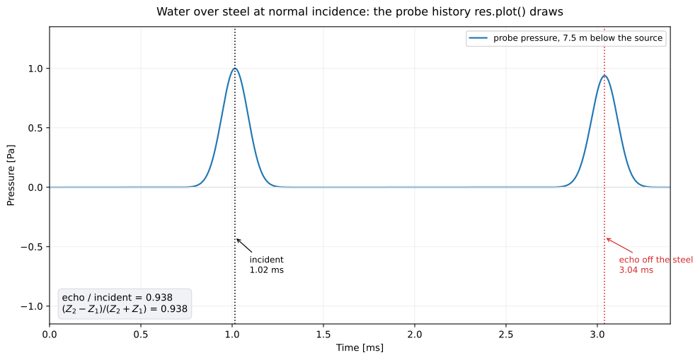
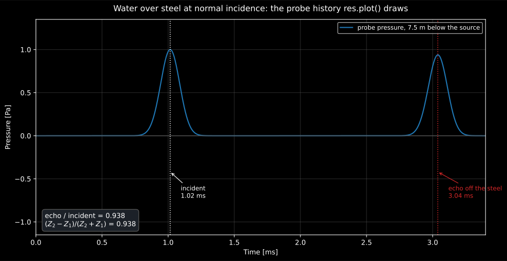
Pressure history at a probe in a 12 metre water column over a steel half-space, over 3.4 milliseconds: a single clean Gaussian pulse of unit amplitude passing the probe at 1.02 milliseconds on its way down, a flat quiet stretch, and a second pulse of the same polarity and 0.938 times the amplitude at 3.04 milliseconds, the reflection returning from the steel, with both arrival times marked and the ratio annotated against the closed-form impedance formula

The whole measurement on one axis. The probe sits 7.5 m below the source and 7.5 m above the contact, so the incident pulse passes it at 1.02 ms and the reflection returns at 3.04 ms — both times fixed by the geometry and the 1480 m/s of water, and both worth checking before the amplitudes are read. The two events keep the same polarity, which is what a reflection off a harder medium does, and their ratio is 0.938 against the exact $(Z_{2} - Z_{1}) / (Z_{2} + Z_{1}) = 0.938$ . The flat stretch between them is the evidence that nothing else in the domain is contributing.

Show the code for this figure

import matplotlib.pyplot as plt

# The run above, re-read: `res.plot()` on a frozen result draws this
# directly. Here the trace was accumulated by hand, so plot it by hand.
plt.plot(t * 1e3, trace)
plt.axvline((4.5025 - 3.0) / WATER.c_p * 1e3, ls=":")   # incident, 1.02 ms
plt.axvline((3.0 + 1.4975) / WATER.c_p * 1e3, ls=":")   # echo, 3.04 ms
plt.xlabel("Time [ms]")
plt.ylabel("Pressure [Pa]")
plt.show()

5. Oblique incidence: mode conversion

Away from normal incidence the solid stops being a liquid. The incident sound refracts into two transmitted waves, P and SV (mode conversion), and refraction obeys Snell’s law separately for each of them, so each has its own critical angle: $arcsin (c_{1} / c_{P 2})$ for the compressional wave and $arcsin (c_{1} / c_{S 2})$ for the shear wave. Both follow from the wave speeds alone — density enters only the amplitudes — so they are two lines of arithmetic on the material constants of section 4.

import numpy as np

# The two critical angles come out of the speeds alone. Substitute your
# own Material pair and the same two lines answer for it.
print(round(float(np.degrees(np.arcsin(WATER.c_p / STEEL.c_p))), 1))   # 14.5
print(round(float(np.degrees(np.arcsin(WATER.c_p / STEEL.c_s))), 1))   # 27.5

The drawing below carries the three arrangements this and the next two sections describe, on one interface line and at three incidences, together with the thing an off-by-one row error gets wrong: where the contact physically sits on the staggered grid.

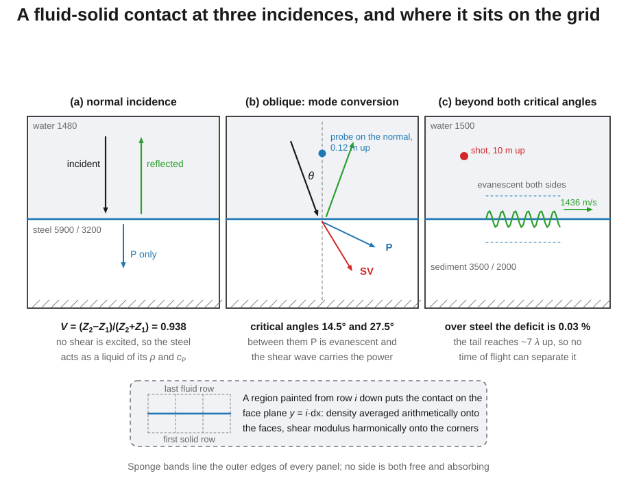
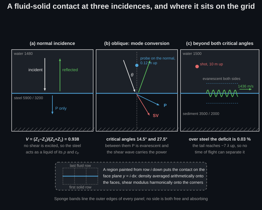
Those two angles cut the range into four regimes. The column headed equivalent fluid is the same interface modelled as a shear-free bottom of the same $c_{P}$ and $ρ$ — the model the underwater module carries — and the difference between the two columns is the whole reason this solver exists.

Incidence	Transmitted waves	\|V\| elastic	\|V\| equivalent fluid	What it means
0°	P only	0.938	0.938	no shear is excited, so the steel is exactly a liquid of its $ρ$ and $c_{P}$
0° to 14.5°	P and SV	0.938 falling to 0.937 at 9°, then rising to the critical angle	0.938 rising to 1	shear already takes a share of the transmitted power, and the fluid model already returns more
14.5° to 27.5°	SV only, P evanescent	dips to 0.905 at 16.4°, 0.918 at 20°	1 (total reflection)	the fluid model over-predicts the returned energy by the whole shear leak
beyond 27.5°	none propagating	1, with a phase	1, with a different phase	total reflection either way; the phase difference is what a Scholte wave locks onto

Read the third row twice: between the critical angles an equivalent fluid reflects everything, while the real interface leaks close to a tenth of the amplitude into a shear wave (|V| falls to 0.905 at 16.4°). The validation suite launches oblique carrier beams at 10° and 20° and matches the exact reflection coefficient of Brekhovskikh & Godin (Eqs. 4.2.22-4.2.26) within a fraction of a percent, mode conversion included, so the elastic column above is measured and not only computed.

How that measurement is made, because it is a technique worth stealing. A tilted Gaussian-carrier beam is written as an initial condition on txx and tyy, with the leapfrog-consistent particle velocity half a time step back split into vx and vy by $sin θ$ and $cos θ$ — the same one-way trick section 4 uses at normal incidence, rotated. The scene is then run twice: once with the solid painted, once with the fluid continued straight through it, and the reference run is forced onto the same time step by scaling its Courant number by $c_{water} / c_{steel}$ so the two traces subtract sample by sample. The difference is the reflected field alone, side-wall artefacts included — the elastic analogue of the ISO 13472-1 subtraction technique. The probe sits directly above the point where the beam axis meets the interface, 0.12 m up, so the incident and reflected beam centres cross it at symmetric transverse offsets and the envelope cancels in the ratio; $∣ V ∣$ is then the amplitude-weighted spectral ratio over the carrier band, not a peak-to-peak reading.

The drawing above is a ray diagram: it says where each wave goes. What a ray cannot say is what “P evanescent” looks like, and that is the whole of the third row of the table. The clip below runs the scene three times, at one incidence from each of the first three regimes — 10°, below both critical angles; 20°, between them; 35°, past the shear one — on the same WATER and STEEL half-space, driving a sustained phase-graded beam onto the contact. Read it as a picture of the regimes, not as a second measurement: each panel is annotated with the closed-form $∣ V ∣$ from the table above, because the beam a 90 mm panel can hold is six wavelengths wide, and at that width the probe sits in the source’s near field rather than in a formed beam. Widening it until a reading is trustworthy would take a panel four times as wide, in which the fringes are too fine to see. The measured column of the table comes from the validation suite instead, which has the room to do it properly.

Download the animation (WebM)

At 10° two beams leave the contact along the dashed Snell directions, and they leave at different angles because they travel at different speeds — the slower shear wave plunging at 22.1° from the normal, the faster compressional wave bent much further out, to 43.8°. At 20° the P beam is not a shallower beam: it is gone. What stands in its place is a skin that clings to the contact and dies within a wavelength, carrying nothing downward, while the shear beam alone takes what crosses — and that shear leak is why the reflection settles at 0.918 rather than the 1.000 an equivalent fluid would return. At 35° both are evanescent and nothing propagates away into the steel: what fills the solid there is an inhomogeneous wave running along the contact and dying with depth, bright and going nowhere. Above the contact, meanwhile, the incident beam and a reflection that is total in amplitude but shifted in phase resolve into a standing pattern. That phase is what the next section builds a Scholte wave out of.

Each panel draws its steel half with its own annotated display gain, and the reason is worth knowing: water drives steel through a thirtyfold impedance step, so the transmitted field carries a small particle velocity even where it carries real power — and the three panels are unlike each other in a way no single gain spans. At 10° the transmitted energy leaves in two beams, so the amplitude anywhere is small; at 35° nothing leaves at all and the evanescent field piles up against the contact, bright and going nowhere. Brightness in the steel is therefore not power. Read the printed $∣ V ∣$ , and the gain factor on each panel, for that.

This is exactly the shear physics that the fluid-bottom reflection_coefficient of the underwater module cannot represent, and the reason a shear-supporting seabed loses more energy than its equivalent-fluid model.

6. The Scholte interface wave

Total reflection beyond the S critical angle leaves both media carrying only evanescent fields, and those fields can lock together into a true interface wave: the Scholte wave, the fluid-solid analogue of the Rayleigh wave. It travels slower than both the fluid sound speed and the solid shear speed, has no low-frequency cut-off and does not disperse over homogeneous half-spaces; scholte_speed solves its exact characteristic equation (B&G Eq. 4.4.20).

from phonometry.simulation import Material, STEEL, WATER, scholte_speed

print(round(scholte_speed(WATER, STEEL), 1))       # 1479.6, 0.03 % below water
seabed = Material(c_p=3500.0, c_s=2000.0, rho=2500.0)
print(round(scholte_speed(Material(1500.0, 0.0, 1000.0), seabed), 1))  # 1436.0

The two cases use different water on purpose. WATER is the library constant at 1480 m/s, while the sediment case follows the van Vossen benchmark, whose fluid is 1500 m/s — so the two deficits below, 0.03 % and 4 %, are each measured against their own fluid, and 1436 m/s should never be compared with 1480 m/s.

Those two numbers tell the whole story. Over a stiff bed (steel) the Scholte wave hugs the water speed (1480 m/s) to within 0.03 % and its evanescent tail reaches ~7 wavelengths up into the water: it is essentially a grazing water wave and cannot be separated by time of flight in any reasonable domain (over air-solid contacts the deficit collapses to ~ $1 0^{- 12}$ of $c$ and the wave is unobservable outright). Over a soft sediment the speed drops well below the water speed and the wave squeezes to within half a wavelength of the contact, which is why measured seabed interface waves are a standard probe of sediment shear speed. The snapshot below runs that soft case: an explosive shot just above the bottom, and the strongest late feature is the interface-hugging Scholte train, timed by the test suite at 1436 m/s within 2 % between two contact probes.

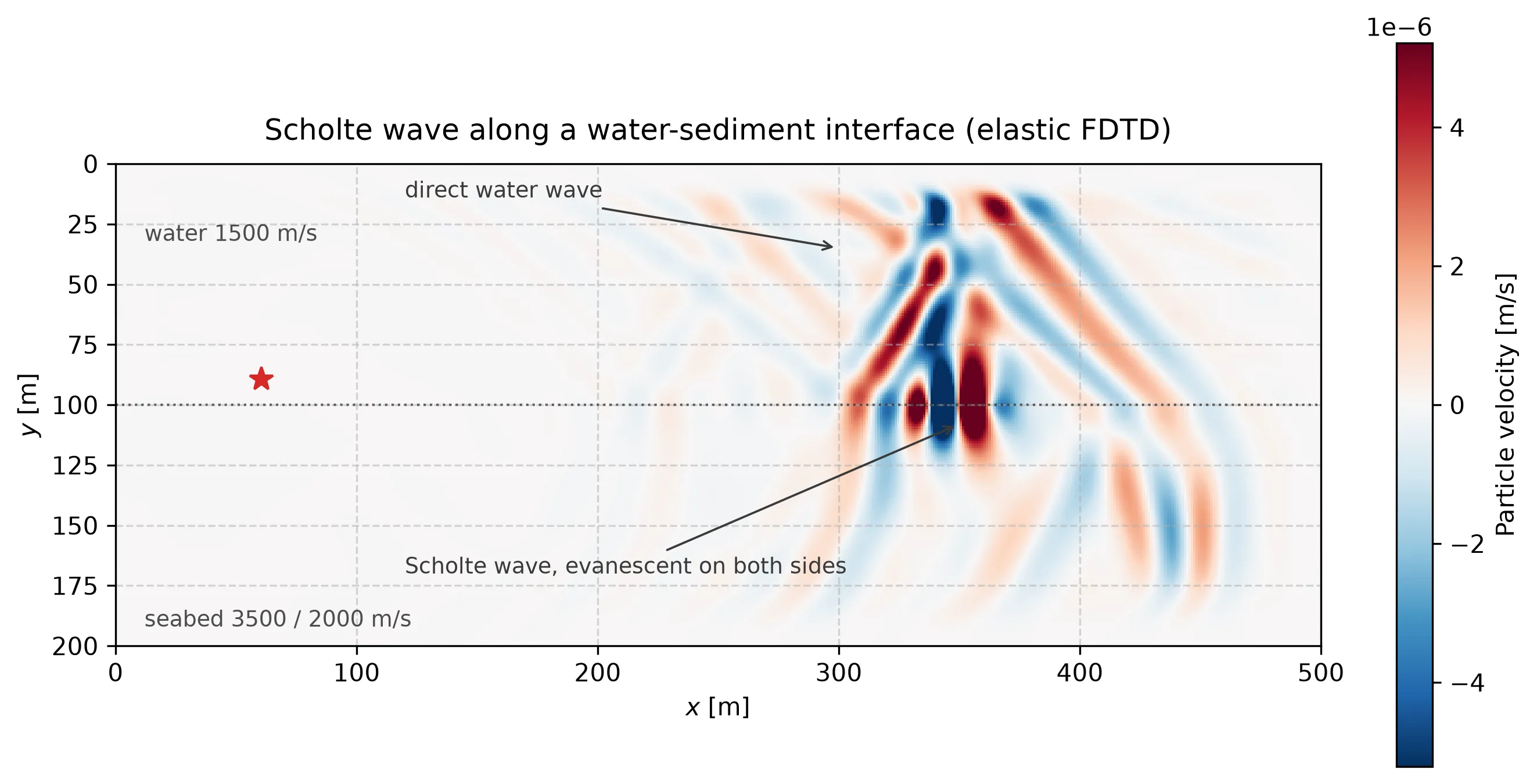
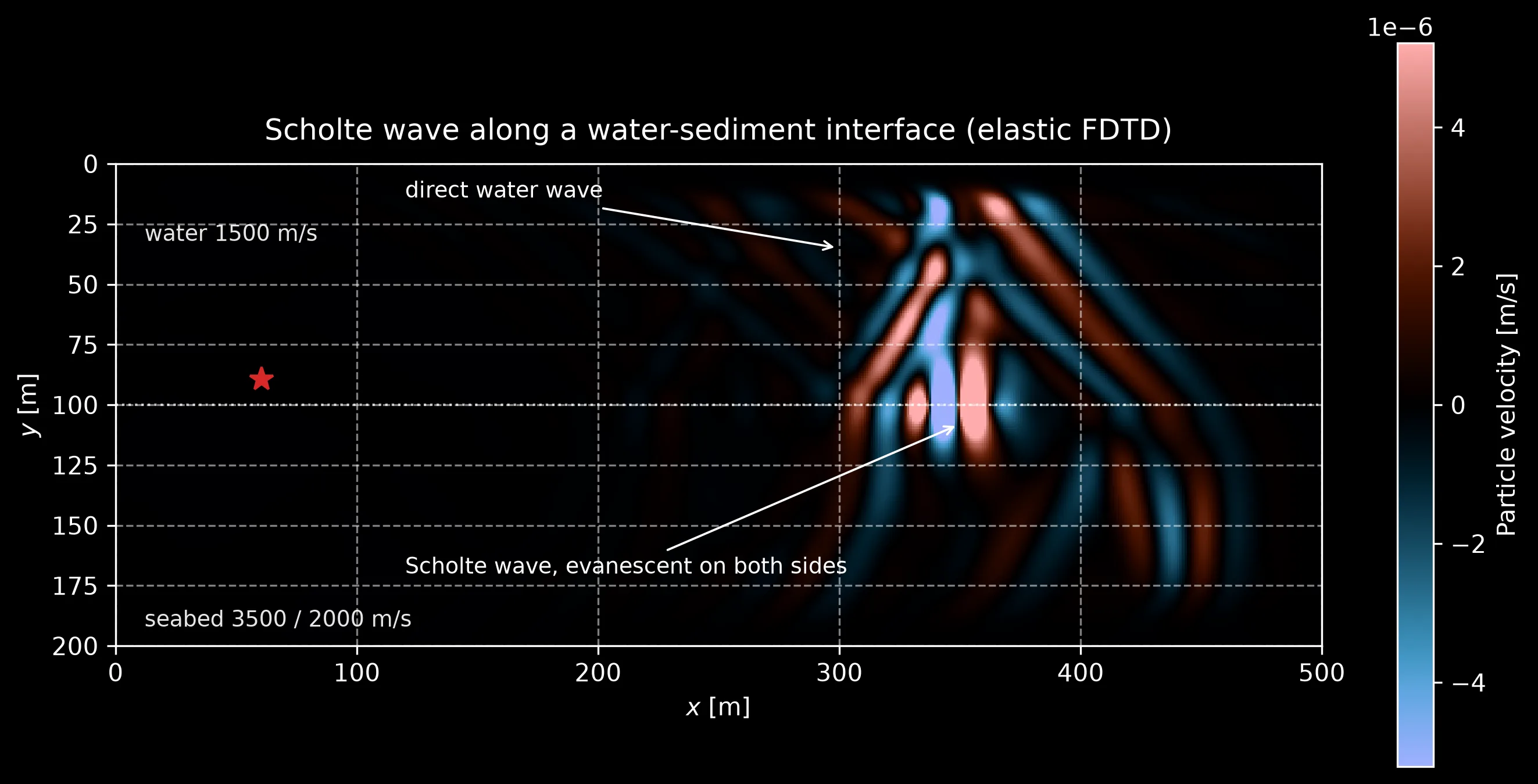
Snapshot of the vertical particle velocity in a 500 by 200 metre domain of water over a soft sediment half-space, 0.2 seconds after an explosive shot 10 metres above the contact: the direct water wavefront arcs up and to the right, oblique wavefronts radiate into the sediment, and the strongest lobes form a compact train hugging the dotted interface line, labelled as the Scholte wave, evanescent on both sides

The van Vossen benchmark media (water over a 3500/2000/2500 sediment): the Scholte train crawls along the contact at 1436 m/s, evanescent into both media, while the direct water wave runs ahead at 1500 m/s.

Show the code for this figure

import numpy as np
import matplotlib.pyplot as plt
from phonometry import simulation

# Water over a soft seabed; explosive 50 Hz Ricker 10 m above the contact.
ny, nx, dx = 200, 500, 1.0
c_p = np.full((ny, nx), 1500.0)
c_s = np.zeros((ny, nx))
rho = np.full((ny, nx), 1000.0)
c_p[100:], c_s[100:], rho[100:] = 3500.0, 2000.0, 2500.0
f0, t0 = 50.0, 0.030
dt = 0.6 * dx / (3500.0 * np.sqrt(2.0))
steps = round(0.232 / dt)

def ricker(t):
    a = (np.pi * f0 * (t - t0)) ** 2
    return (1.0 - 2.0 * a) * np.exp(-a)

res = simulation.elastic_fdtd_simulation(
    c_p, c_s, dx, 0.232, rho=rho,
    sources=[simulation.ExplosionSource(ix=60, iy=89, waveform=ricker,
                                        amplitude=1e3)],
    boundaries=simulation.ElasticBoundaries("absorbing",
                                            absorbing_layer_cells=20),
    recording=simulation.ElasticRecording(snapshot_every=steps,
                                          snapshot_field="vy"),
)
res.plot(kind="snapshot")
plt.show()

7. Immersed plates and the mass law

An immersed plate closes the loop with the building-acoustics module. At normal incidence no shear is excited, so an elastic plate in water is exactly the three-media fluid layer of B&G §2.4: its transmission follows the closed form of Eq. 2.4.14, which reduces to the familiar mass law for thin plates and low frequencies and predicts total transmission at the half-wave thickness resonances $f_{n} = n c_{P} / (2 h)$ (Eq. 2.4.19). For a 10 mm steel plate that first resonance sits at 295 kHz, and one broadband FDTD run reproduces the whole curve: 5.8 dB at 10 kHz (where mass_law_transmission_loss with water as the ambient fluid agrees with the exact form to 0.02 dB), 18.1 dB at 50 kHz, and a transmission-loss dip within 0.1 % of the 295 kHz resonance. The same suite stress-tests the extreme contrast of an air-steel contact (impedance ratio ~ $1 0^{5}$ :1): stable over 10 000 steps with the reflected amplitude conserved to 0.5 %.

Setup drawing of the immersed-plate transmission run. On the left, a tall narrow vertical strip drawn to scale: 0.75 metres of water with a 10 millimetre steel plate at 0.35 metres, a one-way plane pulse launched downward at 0.25 metres, probe A 30 millimetres above the plate and probe B 50 millimetres below it, with a note that the strip is three cells wide, a one-dimensional problem run in a two-dimensional solver at half a millimetre per cell. On the right, the two probe traces on a common time axis from 0 to 160 microseconds: probe A shows the incident pulse at 47 microseconds inside a shaded 65 microsecond gate and its plate reflection at 88 microseconds outside it, probe B shows only the transmitted ring-down. Below them the transmission-loss formula, and a boxed sketch of the half-wave standing pattern inside the plate with the 295 kilohertz first resonance.

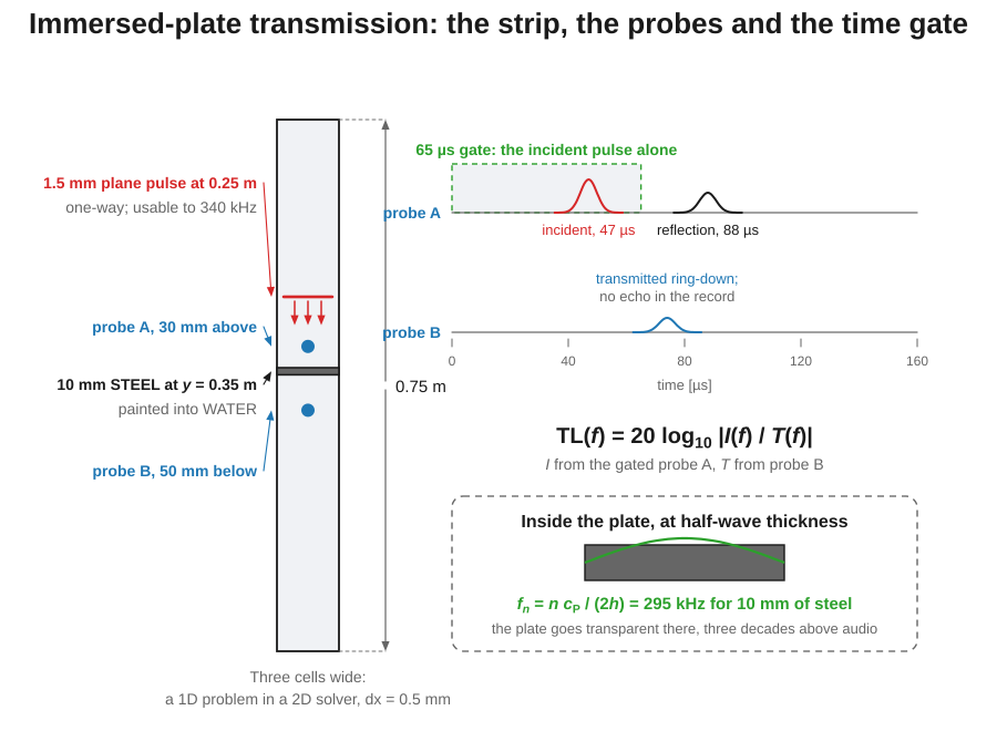
The measurement behind those three numbers. The scene is a strip three cells wide and 0.75 m tall at $Δ x = 0.5$ mm — a one-dimensional problem run in a two-dimensional solver — filled with WATER, with a 10 mm STEEL region painted at 0.35 m by from_regions. A Gaussian plane pulse 1.5 mm wide is written one-way as in section 4, centred at 0.25 m; that width is what carries usable energy out to about 340 kHz, which is what puts the 295 kHz resonance inside the measured band. One probe sits 30 mm above the plate and one 50 mm below its lower face, and the run lasts 0.45 ms.

The measurement itself is a time gate, and the geometry hands you the gate for free. The upper probe sees the incident pulse at about 47 µs (0.07 m of water at 1480 m/s) and its plate reflection at about 88 µs (0.13 m); both arrivals are roughly 10 µs long, so a 65 µs gate isolates the incident one exactly rather than approximately. The lower probe stays echo-free for the whole record, so it needs no gate at all. Then $TL (f) = 20 lo g_{10} ∣ I (f) / T (f) ∣$ from the two magnitude spectra. Two checks a reader can run on their own plate: the 10 kHz value against mass_law_transmission_loss with water as the ambient fluid, and the dip against $f_{n} = n c_{P} / (2 h)$ . The same time-gating logic is what an in-situ ISO 13472-1 measurement does with an Adrienne window, so the trick transfers straight to a real bench.

What the 295 kHz is actually for. It is three decades above the building-acoustics band, so an audio-frequency panel is always in the thin-plate limit, where the layer’s transmission collapses onto the mass law and the thickness resonance can be ignored entirely — which is exactly why the closed forms of the panel-insulation guide never mention it. The resonance earns its keep in its own band: total transmission at half-wave thickness is the principle behind ultrasonic thickness gauging and behind the choice of transducer coupling layers, which is why the validation deliberately drives the plate to hundreds of kilohertz. The frequency where the two regimes meet is one division for any plate: $c_{P} / (2 h)$ , which is 295 kHz for 10 mm of steel and 59 kHz for 50 mm of it.

At oblique incidence the plate physics gets richer, and the clip below is this solver driving the same 10 mm steel plate, now lying in air, with a sustained 45° plane wave arriving on it. The two panels differ in one number only — the drive frequency, $f_{c} /2 = 603$ Hz on the left and $2 f_{c} = 2413$ Hz on the right, either side of the 1206 Hz coincidence frequency the library computes from the same $m^{''}$ and $B^{'}$ used above. Everything else, the plate, the angle, the mesh and the colour scale, is held fixed. Below $f_{c}$ the plate reflects almost everything and the transmitted level lands on the oblique mass law; above it the acoustic trace wavelength matches the free bending wavelength, the plate re-radiates a 45° beam that grows along the lit span, and the transmitted level holds at the low-frequency figure where the mass law demanded 12 dB more blocking. The air below the plate is drawn on both panels with the display gain _weak_field_gain measures off the settled field of the two runs together (×150, that is +44 dB) and prints on the canvas: read the annotations for levels, not the brightness. The panel sound insulation guide takes the same run apart against the plateau method and the mass law.

Download the animation (WebM)

What this guide covers

Covered
The elastic P-SV companion of the acoustic FDTD solver: the Virieux (1986) velocity-stress scheme with the Moczo et al. (2007) effective parameters and stress-imaging free surface, exposed through elastic_fdtd_simulation/ElasticFDTD2D with ExplosionSource and ForceSource, validated against the body-wave speeds, the exact Rayleigh root, the Kirchhoff flexural dispersion and the bit-exact acoustic limit. The fluid-solid coupling of sections 4-7, with the Material constants, ElasticFDTD2D.from_regions and scholte_speed: oblique reflection with mode conversion against Brekhovskikh & Godin (Eqs. 4.2.22-4.2.26) at sub-critical and between-critical angles, the Scholte-wave speed against the exact characteristic equation (Eq. 4.4.20) and by time of flight in the van Vossen (2002) soft-bed benchmark, the immersed-plate transmission with its first thickness resonance against the three-media closed form (Eqs. 2.4.14-2.4.19), the immersed-panel mass law and the air-steel extreme-contrast stress test.
Not covered
Everything the 2D acoustic solver cannot do, this one cannot either: the domain is a cross-section (cylindrical $1/ r$ spreading, not $1/ r$ ), so absolute levels and decay rates are not those of a 3D problem. The solid is isotropic and purely elastic: no anisotropy and no viscoelastic damping beyond the bulk decay rate, so material loss factors are not modelled. There is no elastic perfectly matched layer: the sponge absorbs grazing Rayleigh waves less effectively than body waves. Guided-wave dispersion beyond the thin-plate Kirchhoff regime (full Lamb modes) is observable in the fields but has no dedicated closed-form oracle here.

Quick answers

When do I need the elastic solver instead of the acoustic one?

Whenever any part of the domain supports shear: mode conversion at oblique incidence, Rayleigh waves on free surfaces, Scholte waves at fluid-solid contacts and plate transmission all need the elastic equations. If every cell is fluid, use the acoustic solver: with a uniform c_s = 0 map the elastic solver reproduces it bit for bit, at roughly twice the memory and stepping cost.

What grid resolution does an elastic simulation need?

Resolve at least 10 cells per shortest wavelength using the slowest wave speed in the domain — the slowest non-zero shear speed or a slower fluid sound speed if one is present — $Δ x \leq c_{min} / (10 f)$ . Allow 15-20 cells per wavelength along free surfaces (the stress-imaging boundary is the most dispersive part of the scheme), and at least 15 points per wavelength when an interface wave has to be timed (van Vossen et al. 2002).

What is a Scholte wave and how fast does it travel?

The Scholte wave is the true interface wave of a fluid-solid contact: evanescent into both media, elliptical particle motion, no low-frequency cut-off and non-dispersive over homogeneous half-spaces. Its speed solves the exact characteristic equation (Brekhovskikh & Godin Eq. 4.4.20, scholte_speed) and always lies below both the fluid sound speed and the solid shear speed: 0.03 % below the water speed (1480 m/s) over steel (1479.6 m/s), but 4 % below the 1500 m/s ocean water of the sediment example (1436 m/s for that water over a 3500/2000/2500 bed), which is why seabed interface waves probe the sediment shear stiffness.

References

Brekhovskikh, L. M., & Godin, O. A. (1990). Acoustics of layered media I: Plane and quasi-plane waves. Springer. https://doi.org/10.1007/978-3-642-52369-4The fluid-solid oracles of sections 4-7: the oblique reflection coefficient with mode conversion (Eqs. 4.2.22-4.2.26) and its critical-angle limits (Eqs. 4.2.27-4.2.31), the exact Scholte characteristic equation (Eqs. 4.4.18-4.4.20) with the light-fluid asymptotics (Eqs. 4.4.21-4.4.24), and the three-media layer transmission (Eqs. 2.4.10-2.4.19).
Cremer, L., Heckl, M., & Petersson, B. A. T. (2005). Structure-borne sound (3rd ed.). Springer. https://doi.org/10.1007/b137728The analytic oracles of the elastic solver: the exact Rayleigh characteristic equation (Eq. 3.149) and the Kirchhoff flexural dispersion with its thickness correction (Eqs. 3.83-3.89, 3.196b).
Moczo, P., Kristek, J., Galis, M., Pazak, P., & Balazovjech, M. (2007). The finite-difference and finite-element modeling of seismic wave propagation and earthquake motion. Acta Physica Slovaca, 57(2), 177-406. The heterogeneous effective grid parameters of section 2 (harmonic shear modulus, arithmetic density; Eqs. 7.37-7.39) and the stress-imaging free surface of section 3 (Eq. 9.9).
van Vossen, R., Robertsson, J. O. A., & Chapman, C. H. (2002). Finite-difference modeling of wave propagation in a fluid-solid configuration. Geophysics, 67(2), 618-624. https://doi.org/10.1190/1.1468623The fluid-solid benchmark of the same staggered scheme: the harmonic shear modulus and arithmetic density averages (Eqs. 9-10) that satisfy the interface conditions implicitly, the soft-bed configuration of the Scholte case of section 6 and the >= 15 points-per-wavelength rule for the O(2,2) scheme with an interface wave.
Virieux, J. (1986). P-SV wave propagation in heterogeneous media: velocity-stress finite-difference method. Geophysics, 51(4), 889-901. https://doi.org/10.1190/1.1442147The elastic solver of section 1: the velocity-stress system (Eq. 2), the fully staggered cell and update (Fig. 1, Eq. 5), the P-only Courant bound (Eqs. 6-7), the dispersion relations (Eqs. 13-14) and the liquid as the shear-free limit.

Created and maintained by José Manuel Requena Plens ORCID All projects

Elastic waves and fluid-solid coupling

1. The P-SV velocity-stress scheme

2. Fluids inside the elastic solver

3. Free surfaces and Rayleigh waves

4. Fluid-solid coupling at normal incidence

5. Oblique incidence: mode conversion

6. The Scholte interface wave

7. Immersed plates and the mass law

What this guide covers

See also

Quick answers

When do I need the elastic solver instead of the acoustic one?

What grid resolution does an elastic simulation need?

What is a Scholte wave and how fast does it travel?

References